Cryptocurrency Market Clustering with Affinity Propagation in Python

Affinity propagation can reveal groups of cryptocurrencies whose returns moved similarly, without requiring us to choose the number of clusters first. This tutorial analyzes daily returns for 12 large cryptocurrencies from January 2023 through December 2025. It also estimates a sparse partial-correlation network and places the assets on a two-dimensional market map.

The executed example identifies five clusters. Bitcoin, Ethereum, Solana, and Dogecoin form one group. Cardano, Polkadot, Litecoin, Chainlink, and Avalanche form another. BNB, XRP, and Bitcoin Cash are singleton clusters in this sample.

The complete, executed notebook is available in the Relataly Python tutorials repository.

Disclaimer

This tutorial is for educational purposes and does not constitute financial advice. The clusters describe historical co-movement in a selected sample. They do not predict returns or establish causal relationships.

What Is Affinity Propagation?

Affinity propagation is an unsupervised clustering algorithm that exchanges two kinds of messages between observations:

• Responsibility measures how suitable one observation is as another observation’s exemplar.
• Availability measures how appropriate it would be for an observation to select a candidate exemplar.

The algorithm iterates until a set of exemplars and their associated clusters stabilizes. Affinity propagation does not need a predefined cluster count. Its result depends on the similarity matrix, preference values, damping, and sample data.

Pairwise Pearson correlation between daily log returns serves as the similarity measure in this analysis. A high positive correlation means that two assets tended to move in the same direction on the same day during the sample window.

Analysis Workflow

The workflow has five stages:

1. Download adjusted daily prices for a fixed set of cryptocurrency tickers.
2. Convert prices to daily log returns and verify asset-label alignment.
3. Cluster the return-correlation matrix with affinity propagation.
4. Estimate sparse partial correlations with graphical lasso.
5. Visualize the full correlation matrix and the strongest conditional relationships.

Prerequisites

The tutorial uses Python 3.12 with pandas, NumPy, matplotlib, seaborn, yfinance, and scikit-learn. Install the packages with:

pip install pandas numpy matplotlib seaborn yfinance scikit-learn

Step 1: Load and Prepare Cryptocurrency Prices

We use a fixed period ending on January 1, 2026. Because yfinance treats its end argument as exclusive, the data covers January 1, 2023 through December 31, 2025.

Downloading each ticker separately makes missing assets visible and avoids assumptions about multi-index column layouts. The code retains assets with returned data, aligns their names to the price columns, forward-fills short gaps, and removes incomplete dates.

import numpy as np
import pandas as pd
import yfinance as yf

ASSETS = {
    "BTC-USD": "Bitcoin",
    "ETH-USD": "Ethereum",
    "BNB-USD": "BNB",
    "XRP-USD": "XRP",
    "ADA-USD": "Cardano",
    "SOL-USD": "Solana",
    "DOGE-USD": "Dogecoin",
    "DOT-USD": "Polkadot",
    "LTC-USD": "Litecoin",
    "LINK-USD": "Chainlink",
    "AVAX-USD": "Avalanche",
    "BCH-USD": "Bitcoin Cash",
}

close_prices = {}
for ticker in ASSETS:
    history = yf.download(
        ticker,
        start="2023-01-01",
        end="2026-01-01",
        auto_adjust=True,
        multi_level_index=False,
        progress=False,
    )
    if not history.empty:
        close_prices[ticker] = history["Close"]

prices = pd.DataFrame(close_prices).sort_index().ffill().dropna()
asset_names = pd.Series(
    {ticker: ASSETS[ticker] for ticker in prices.columns},
    name="asset",
)
returns = np.log(prices).diff().dropna()

assert returns.columns.equals(asset_names.index)
assert np.isfinite(returns.to_numpy()).all()

The executed dataset contains 1,095 daily return observations for all 12 assets.

Step 2: Compare Relative Price Performance

Raw cryptocurrency prices have very different scales. Rebasing every series to 100 makes cumulative performance comparable in one chart.

rebased_prices = prices.div(prices.iloc[0]).mul(100).rename(columns=asset_names)

fig, ax = plt.subplots(figsize=(12, 6))
rebased_prices.plot(ax=ax, linewidth=1, alpha=0.85)
ax.set(
    title="Relative cryptocurrency performance, 2023-2025",
    xlabel=None,
    ylabel="Growth of 100 USD",
)
ax.legend(ncol=3, frameon=False, fontsize=9)
fig.tight_layout()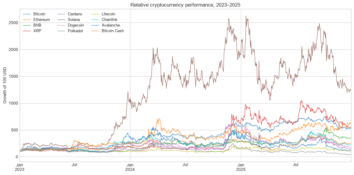

Solana records the strongest cumulative gain in this window, along with substantial volatility. The model uses daily log returns to compare co-movement across differently priced assets.

Step 3: Cluster the Return Correlations

We calculate the Pearson correlation matrix and pass it to AffinityPropagation as a precomputed similarity matrix. A damping value of 0.8 reduces oscillation during message updates. The random state makes tie handling reproducible.

from sklearn.cluster import AffinityPropagation

correlation = returns.corr()
affinity_model = AffinityPropagation(
    affinity="precomputed",
    damping=0.8,
    random_state=42,
).fit(correlation.to_numpy())

labels = affinity_model.labels_

The five clusters from the executed notebook are:

Cluster	Exemplar	Members	Mean within-cluster correlation
1	Bitcoin	Bitcoin, Ethereum, Solana, Dogecoin	0.722
2	BNB	BNB	N/A
3	XRP	XRP	N/A
4	Polkadot	Cardano, Polkadot, Litecoin, Chainlink, Avalanche	0.721
5	Bitcoin Cash	Bitcoin Cash	N/A

Singleton clusters have no within-cluster asset pair, so their mean correlation is undefined. They indicate a sufficiently distinct correlation profile under the current settings.

Step 4: Inspect the Correlation Matrix

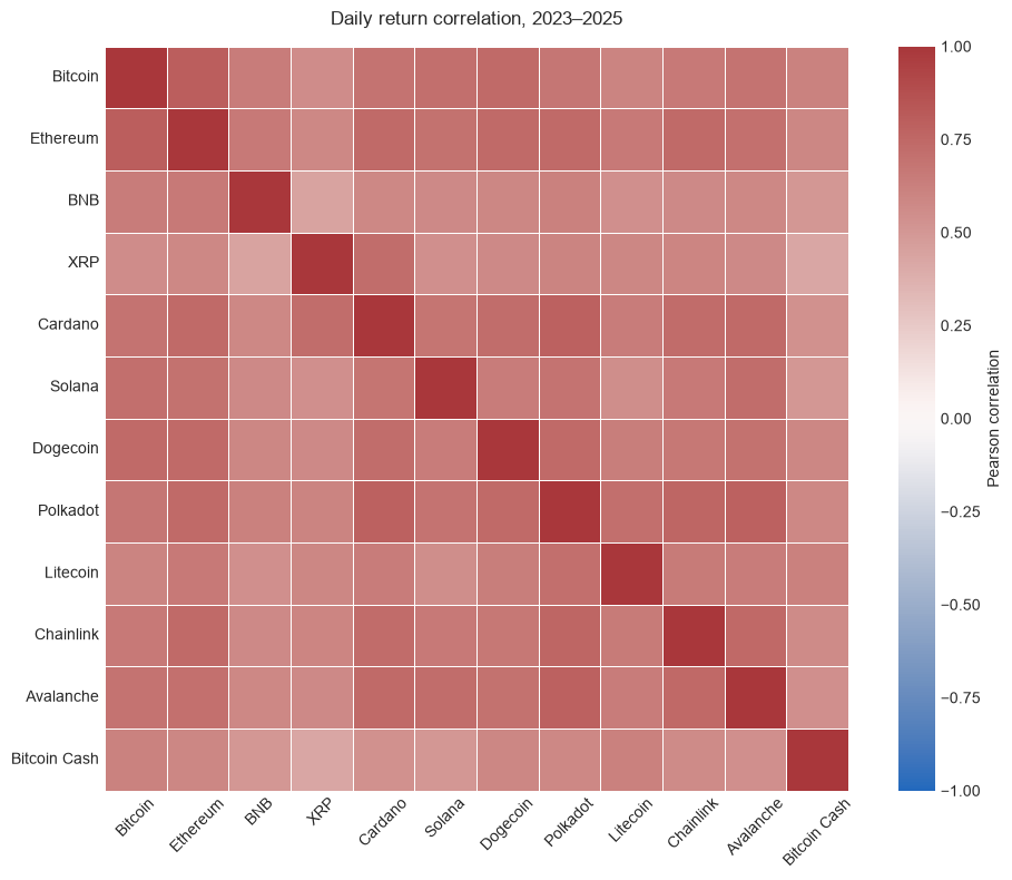
The heatmap shows broad positive co-movement across the sample. It also shows why cluster boundaries are subtle: many pairwise correlations are high, while affinity propagation considers each asset’s complete similarity profile.

display_correlation = correlation.rename(index=asset_names, columns=asset_names)

fig, ax = plt.subplots(figsize=(10, 8))
sns.heatmap(
    display_correlation,
    cmap="vlag",
    center=0,
    vmin=-1,
    vmax=1,
    square=True,
    linewidths=0.5,
    cbar_kws={"label": "Pearson correlation"},
    ax=ax,
)

Step 5: Estimate a Sparse Dependency Network

Ordinary correlation can reflect direct relationships and shared exposure to the broader market. Graphical lasso estimates a sparse precision matrix. Normalized off-diagonal precision values approximate partial correlations after controlling for the remaining assets.

from sklearn.covariance import GraphicalLassoCV
from sklearn.manifold import MDS
from sklearn.preprocessing import StandardScaler

standardized_returns = StandardScaler().fit_transform(returns)
with np.errstate(invalid="ignore"):
    edge_model = GraphicalLassoCV(max_iter=500).fit(standardized_returns)

precision = edge_model.precision_
precision_scale = np.sqrt(np.diag(precision))
partial_correlation = -precision / np.outer(
    precision_scale,
    precision_scale,
)
np.fill_diagonal(partial_correlation, 1.0)

correlation_distance = np.sqrt(
    2 * (1 - correlation.clip(-1, 1))
).to_numpy(copy=True)
np.fill_diagonal(correlation_distance, 0.0)

positions = MDS(
    n_components=2,
    metric="precomputed",
    init="classical_mds",
    normalized_stress="auto",
    random_state=42,
).fit_transform(correlation_distance)

The fitted graphical-lasso regularization parameter is 0.1742. The visualization keeps relationships with an absolute partial correlation of at least 0.107, the larger of 0.05 and the 70th percentile of candidate edge strengths.

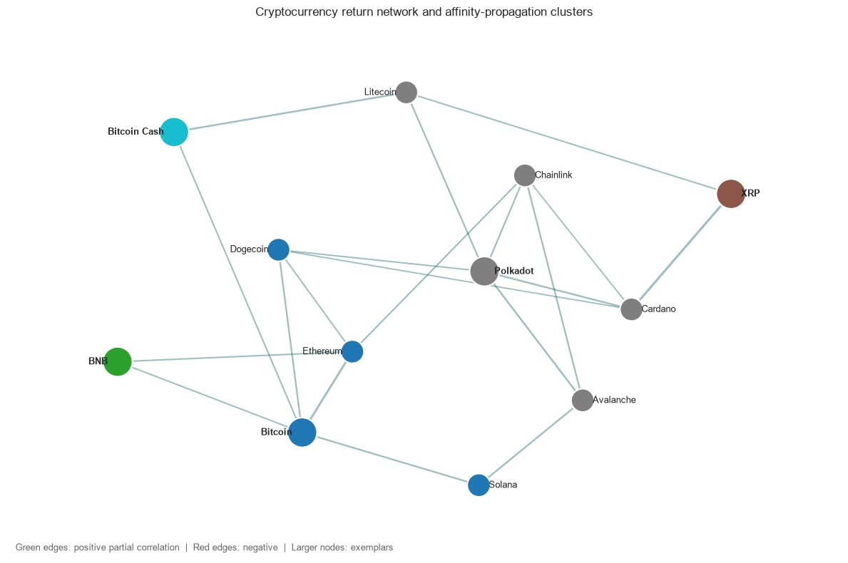
Node color indicates cluster membership. Larger nodes are affinity-propagation exemplars. Green lines show positive partial correlations; the code also supports red lines for negative relationships, although no negative edge passes the threshold in this fitted network. Line width increases with absolute partial-correlation strength.

The two-dimensional positions come from multidimensional scaling of correlation distance. Their axes and orientation have no independent meaning. Distances summarize higher-dimensional relationships with inevitable information loss.

Interpretation and Limitations

The output supports three observations for this sample:

• Bitcoin, Ethereum, Solana, and Dogecoin share a broad correlation profile, with Bitcoin selected as the exemplar.
• Cardano, Polkadot, Litecoin, Chainlink, and Avalanche form a second multi-asset group centered on Polkadot.
• BNB, XRP, and Bitcoin Cash each have a sufficiently distinct similarity profile to become singleton clusters.

These assignments can change when the asset universe, date range, data source, or model preferences change. A larger universe may turn a singleton into part of a new group. A shorter window can make temporary market regimes dominate the result. Data errors, thin trading, and exchange-specific pricing can also distort return correlations.

For a research workflow, repeat the analysis across rolling windows and compare cluster stability. Treat unstable membership as a result to investigate.

Summary

Affinity propagation provides a practical way to explore market structure when the number of groups is unknown. This tutorial used a precomputed return-correlation matrix to cluster 12 cryptocurrencies into five groups. A graphical-lasso model then reduced the dense correlation picture to a sparse network of conditional relationships.

The heatmap, cluster table, and network answer different questions. The heatmap shows pairwise co-movement, the table reports membership and exemplars, and the network highlights stronger conditional links. Together they offer a transparent descriptive view of the selected 2023-2025 market window.

Sources and Further Reading

1. Scikit-learn: AffinityPropagation
2. Scikit-learn: Visualizing the stock market structure
3. Frey and Dueck (2007): Clustering by Passing Messages Between Data Points
4. Friedman, Hastie, and Tibshirani (2008): Sparse Inverse Covariance Estimation with the Graphical Lasso