Feature Engineering for Multivariate Time Series Models with Python

Are you interested in learning how additional features affect a multivariate forecasting model? While a univariate model uses one historical series, a multivariate model can use several inputs to identify patterns and predict future movements. Creating and testing these inputs is known as feature engineering.

In this article, we explore popular financial indicators, including Bollinger position, RSI, moving averages, volatility, and MACD. We calculate them using information available at each session and test whether they improve a one-session-ahead NASDAQ forecast.

But we don’t just stop at theory. We provide a hands-on tutorial using Python to prepare and analyze time-series data for stock market forecasting. We leverage the power of recurrent neural networks with LSTM layers, based on the Keras library, to train and test different model variations with various feature combinations.

By the end of this article, you will know how to create causal technical features, align feature sets on identical dates, avoid preprocessing leakage, and compare the result with both a simpler model and naive benchmarks. The result is useful precisely because the extra indicators do not automatically win.

New to time series modeling? Consider starting with the preceding tutorial on multivariate stock-market forecasting using recurrent neural networks and Python.

Disclaimer: This article does not constitute financial advice. Stock markets can be very volatile and are generally difficult to predict. Predictive models and other forms of analytics applied in this article only illustrate machine learning use cases.

An illustration representing feature engineering for time series analysis, with a laptop displaying financial charts in a study.

Feature engineering transforms historical observations into candidate model inputs. Image generated with Midjourney

Feature Engineering for Stock Market Forecasting - Borrowing Features from Chart Analysis

The idea behind multivariate time series models is to feed the model with additional features that may improve prediction quality. An example is a moving-average distance. Adding more features does not automatically improve predictive performance and increases the time needed to train models. The challenge is to find inputs that add out-of-sample information rather than noise, so we need controlled experiments instead of assuming that established indicators will help.

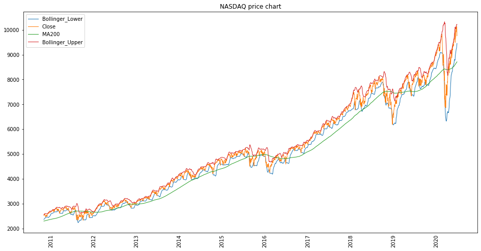
In stock market forecasting, we can borrow indicators from chart analysis. This discipline studies historical prices and trading volume for patterns associated with subsequent movements. A machine learning model does not inspect the chart manually; it receives numerical representations of those patterns. Every representation must use only information available at the prediction time. Feature engineering for multivariate stock market prediction - A multivariate time series forecast. Keras, Scikit-Learn, Python, Tutorial

A multivariate time-series forecast, as we will create it in this article. Exemplary chart with technical indicators (Bollinger bands, RSI, and Double-EMA)

Stock Market Forecasting - Does this really Work?

It is essential to point out that the effectiveness of chart analysis and algorithmic trading is controversial. There is at least as much controversy about whether it is possible to predict the price of stock markets with neural networks. Various studies and researchers have examined the effectiveness of chart analysis with different results. One of the most significant points of criticism is that it cannot take external events into account. Nevertheless, many financial analysts consider financial indicators when making investment decisions, so a lot of money is moved simply because many people believe in statistical indicators.

So without knowing how well this will work, it is worth an attempt to feed a neural network with different financial indicators. But first and foremost, I see this as an excellent way to show how feature engineering works. Just make sure not to rely on the predictions of these models blindly.

Also: Stock Market Prediction using Univariate Recurrent Neural Networks

Selected Statistical Indicators

The following indicators are commonly used in chart analysis and may be helpful when creating forecasting models:

Relative Strength Index
Simple Moving Averages
Exponential Moving Averages
Bollinger Bands

Relative Strength Index (RSI)

The Relative Strength Index (RSI) is one of the most commonly used oscillating indicators. In 1978, Welles Wilder developed it to determine the momentum of price movements and compare the strength of price losses in a period with price gains. It can take percentage values between 0 and 100.

RSI is commonly interpreted relative to 30 and 70: values below 30 are described as oversold, while values above 70 are described as overbought. These thresholds summarize recent momentum; they do not determine when a reversal will happen.

The formula for the RSI is as follows:

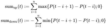
Calculate the sum of all positive and negative price changes in a period (e.g., 30 days):
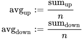
We then calculate the mean value of the sums with the following formula:
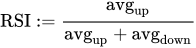
Finally, we calculate the RSI with the following formula:

$feature engineering for stock price prediction: formula for the rsi, Keras, Scikit-Learn, Python, Tutorial$ $feature engineering for stock price prediction: formula for the rsi, Keras, Scikit-Learn, Python, Tutorial$ $feature engineering for stock price prediction: formula for the rsi,Keras, Scikit-Learn, Python, Tutorial$

Simple Moving Averages (SMA)

Simple Moving Averages (SMAs) are technical indicators used to summarize price trends. An SMA is the arithmetic mean of observations within a rolling period. Analysts often inspect 50-day and 200-day averages and describe their crossovers as death or golden crosses.

A death cross occurs when a shorter moving average crosses below a longer moving average.
A golden cross occurs when a shorter moving average crosses above a longer moving average.

We can use the SMA in the input shape of our model simply by measuring the distance between two trendlines.

Exponential Moving Averages (EMA)

The exponential moving average (EMA) is another lagging trend indicator. Like the SMA, the EMA measures the strength of a price trend. The difference between SMA and EMA is that the SMA assigns equal values to all price points, while the EMA uses a multiplier that weights recent prices higher.

Calculating an EMA for a given data point requires past price values. The smoothing multiplier for span $n$ is commonly $2/(n+1)$ , so a 30-session EMA uses a multiplier of approximately 0.0645.

After initialization, each value is calculated as: EMA = current closing price x multiplier + previous EMA x (1 - multiplier).

Bollinger Bands

Bollinger Bands are a popular technical analysis tool used to identify market volatility and potential price movements in financial markets. They are named after their creator, John Bollinger.

Bollinger Bands consist of three lines that are plotted on a price chart. The middle line is a simple moving average (SMA) of the asset price over a specified period (typically 20 days). The upper and lower lines are calculated by adding and subtracting a multiple (usually two) of the standard deviation of the asset price from the middle line.

The upper band is calculated as: Middle band + (2 x Standard deviation) The lower band is calculated as: Middle band - (2 x Standard deviation)

The standard deviation is a measure of how much the asset price deviates from the average. When the asset price is more volatile, the bands widen, and when the price is less volatile, the bands narrow.

Traders sometimes interpret contact with the upper or lower band as an overbought or oversold condition. A band crossing is not a reliable buy or sell signal by itself, which is why this tutorial tests normalized Bollinger position as one candidate feature rather than encoding a trading rule.

Feature Engineering for Time Series Prediction Models in Python

In the following, this tutorial will guide you through the process of implementing a multivariate time series prediction model for the NASDAQ stock market index. Our aim is to equip you with the knowledge and practical skills required to create a powerful predictive model that can effectively forecast stock prices.

Throughout this tutorial, we will take you through a step-by-step approach to building a multivariate time series prediction model. You will learn how to implement and utilize different features to train and measure the performance of your model. Our goal is to ensure that you are not only able to understand the underlying concepts of multivariate time series prediction, but that you are also capable of applying these concepts in a practical setting.

The code is available on the GitHub repository.

Let's do some feature engineering for machine learning!

Let’s do some feature engineering for machine learning!

Prerequisites

Before starting the coding part, make sure you have set up a Python 3 environment. This version was tested with Python 3.12, TensorFlow 2.21, Keras 3.15, pandas 3.0, NumPy 2.5, scikit-learn 1.9, and yfinance 1.5. The project repository contains the complete dependency list.

TensorFlow 2.11 and later do not use the GPU on native Windows. The model in this tutorial is intentionally compact and runs on a CPU; WSL2 is an option if you need CUDA support.

Step #1 Load the Data

Let’s start by setting up the imports and loading the data. Our Python project will use price data from the NASDAQ composite index (symbol: ^IXIC) from yahoo.finance.com.

# Time Series Forecasting - Feature Engineering for Multivariate Models
# A tutorial for this file is available at www.relataly.com
# Tested with Python 3.12, TensorFlow 2.21, Keras 3.15, pandas 3.0, and yfinance 1.5

import keras
import matplotlib.dates as mdates
import matplotlib.pyplot as plt
import numpy as np
import pandas as pd
import seaborn as sns
import tensorflow as tf
import yfinance as yf
from sklearn.metrics import mean_absolute_error, root_mean_squared_error
from sklearn.preprocessing import RobustScaler

sns.set_theme(style="white", rc={"axes.spines.right": False, "axes.spines.top": False})
keras.utils.set_random_seed(42)

print(f"TensorFlow version: {tf.__version__}")
print(f"Available GPUs: {len(tf.config.list_physical_devices('GPU'))}")

start_date = "2010-01-01"
end_date = "2026-01-01"
stock_name = "NASDAQ Composite"
symbol = "^IXIC"

df = yf.download(
  symbol,
  start=start_date,
  end=end_date,
  auto_adjust=True,
  multi_level_index=False,
  progress=False,
)
if df.empty:
  raise RuntimeError("yfinance returned no data for the NASDAQ Composite")

print(df.shape)
df.head()

TensorFlow version: 2.21.0
Available GPUs: 0
(4024, 5)

The fixed end date makes the example reproducible. auto_adjust=True gives one consistent adjusted OHLCV schema, while multi_level_index=False prevents a one-symbol download from returning MultiIndex columns in current yfinance versions.

Step #2 Explore the Data

Let’s take a quick look at the data by creating line charts for the columns of our data set.

df_plot = df.copy()
_, axes = plt.subplots(nrows=3, ncols=2, sharex=True, figsize=(14, 9))

for ax, column in zip(axes.flat, df_plot.columns):
  sns.lineplot(x=df_plot.index, y=df_plot[column], ax=ax)
  ax.xaxis.set_major_locator(mdates.AutoDateLocator())
  ax.set_title(column)

for ax in axes.flat[len(df_plot.columns):]:
  ax.set_visible(False)

plt.tight_layout()
plt.show()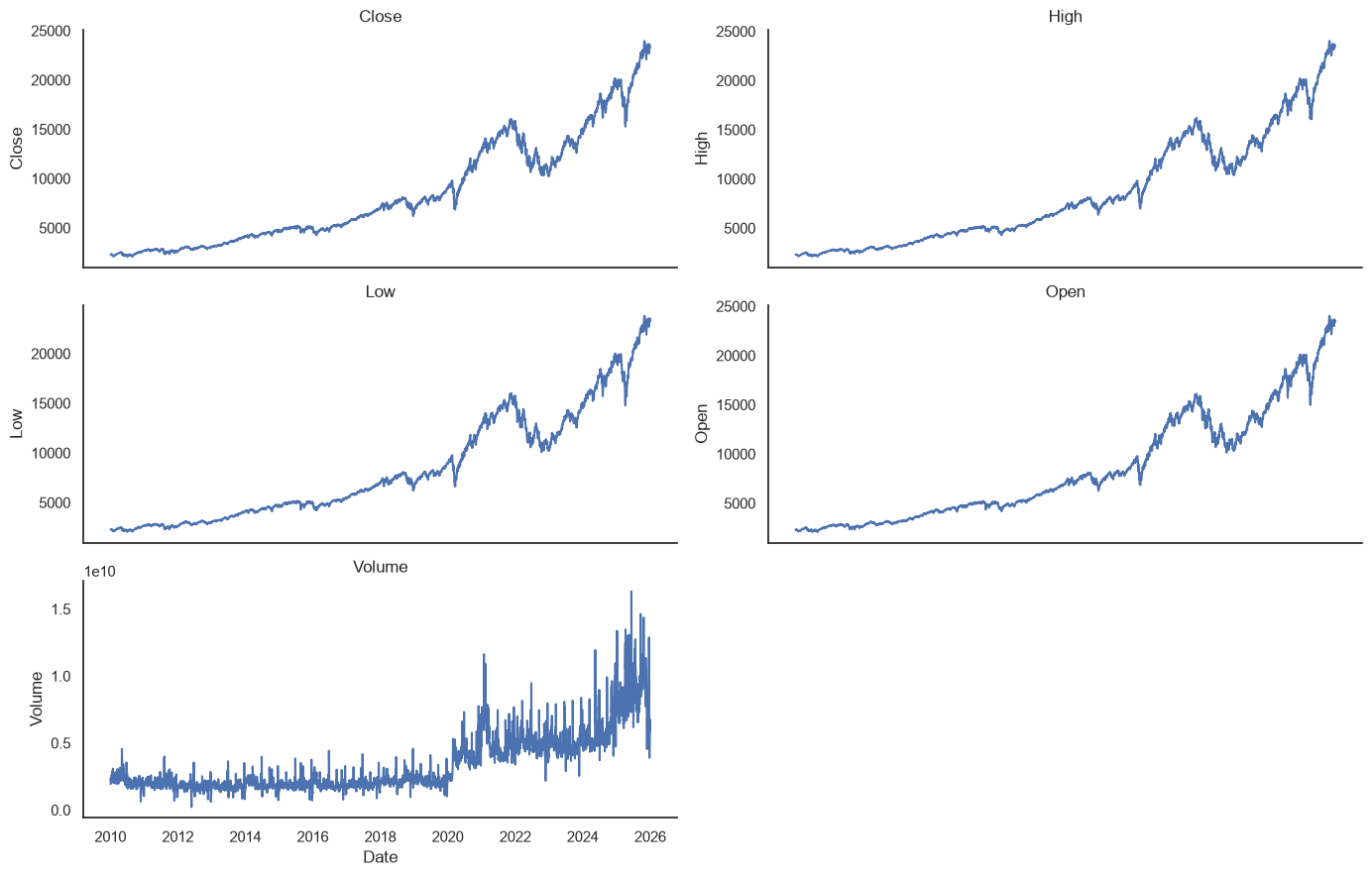

NASDAQ price and volume history used for the feature-engineering comparison

Our adjusted dataset includes five columns: Open, High, Low, Close, and Volume. The price levels trend strongly over time, so we will model stationary log changes instead of asking the network to extrapolate the index level directly.

Step #3 Feature Engineering

Now comes the exciting part: we will implement additional features. The comparison uses two input sets. The baseline contains log changes for adjusted OHLC prices and volume. The engineered set adds eight scale-free technical indicators.

Every feature for session $t$ must be calculable using data available through session $t$ . The sequence ending at $t$ predicts the Close return at $t+1$ . Future shifts such as shift(-1) are therefore invalid input features, even if they make a historical backtest look better.

market = df.sort_index().dropna().copy()
market.tail()

The technical indicators are expressed as ratios or normalized distances. This keeps them comparable as the NASDAQ level changes over the 16-year sample. Rolling features retain their natural missing warm-up period; we drop those rows rather than replacing them with a value from another date.

def create_feature_sets(market):
  price_columns = ["Open", "High", "Low", "Close"]
  price_log_returns = np.log(market[price_columns]).diff()
  volume_log_change = np.log1p(market["Volume"]).diff().rename("Volume")
  baseline = pd.concat([price_log_returns, volume_log_change], axis=1)

  close = market["Close"]
  close_return = price_log_returns["Close"]
  sma20 = close.rolling(window=20).mean()
  sma50 = close.rolling(window=50).mean()
  price_std20 = close.rolling(window=20).std()
  return_volatility20 = close_return.rolling(window=20).std()
  ema12 = close.ewm(span=12, adjust=False).mean()
  ema26 = close.ewm(span=26, adjust=False).mean()

  price_change = close.diff()
  average_gain = price_change.clip(lower=0).ewm(
    alpha=1 / 14,
    adjust=False,
    min_periods=14,
  ).mean()
  average_loss = (-price_change.clip(upper=0)).ewm(
    alpha=1 / 14,
    adjust=False,
    min_periods=14,
  ).mean()
  relative_strength = average_gain / average_loss

  technical = pd.DataFrame(
    {
      "Intraday_Range": np.log(market["High"] / market["Low"]),
      "Open_to_Close": np.log(close / market["Open"]),
      "SMA20_Distance": close / sma20 - 1,
      "SMA50_Distance": close / sma50 - 1,
      "Return_Volatility20": return_volatility20,
      "Bollinger_Position": (close - sma20) / (2 * price_std20),
      "RSI14": (100 - 100 / (1 + relative_strength)) / 100,
      "MACD_Spread": (ema12 - ema26) / close,
    },
    index=market.index,
  )

  engineered = pd.concat([baseline, technical], axis=1)
  engineered = engineered.replace([np.inf, -np.inf], np.nan).dropna()
  baseline = baseline.loc[engineered.index]
  return baseline, engineered


baseline_features, engineered_features = create_feature_sets(market)
assert baseline_features.index.equals(engineered_features.index)
assert np.isfinite(engineered_features.to_numpy()).all()

print(f"Baseline shape: {baseline_features.shape}")
print(f"Engineered shape: {engineered_features.shape}")
print(f"Common dates: {engineered_features.index.min().date()} -> {engineered_features.index.max().date()}")

Baseline shape: (3975, 5)
Engineered shape: (3975, 13)
Common dates: 2010-03-16 -> 2025-12-31

The assertions are important. They verify that both model variants cover exactly the same dates and that no missing or infinite values reach a scaler or neural network. We can now inspect the eight added indicators without mixing their different units on one axis.

technical_columns = [
  column
  for column in engineered_features.columns
  if column not in baseline_features.columns
]
feature_preview = engineered_features.loc["2024-01-01":, technical_columns]
_, axes = plt.subplots(nrows=4, ncols=2, sharex=True, figsize=(14, 11))

for ax, column in zip(axes.flat, technical_columns):
  sns.lineplot(x=feature_preview.index, y=feature_preview[column], ax=ax)
  ax.set_title(column)

plt.tight_layout()
plt.show()
engineered_features.tail()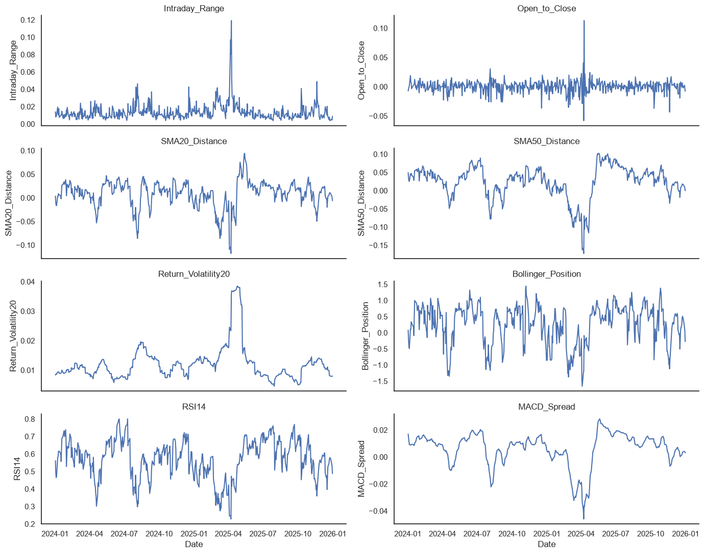

Engineered technical indicators derived from the NASDAQ price and volume history

The plots show that these indicators describe different properties: intraday range and volatility measure dispersion, moving-average and MACD distances describe trend, and RSI and Bollinger position describe where the current price sits relative to recent behavior. Whether those descriptions contain incremental forecasting information remains an empirical question.

Step #4 Scaling and Transforming the Data

Before training our models, we need to scale the features and create chronological sequences. RobustScaler centers each column by its median and scales it using its interquartile range; it does not map values to a fixed range between zero and one.

We first choose the 80% training boundary, then fit every scaler on training rows only. Fitting on the full series would leak the distribution of the test period into preprocessing.

close_returns = baseline_features[["Close"]].to_numpy()
close_levels = market.loc[baseline_features.index, "Close"].to_numpy()
train_size = int(len(baseline_features) * 0.8)

baseline_scaler = RobustScaler()
baseline_scaler.fit(baseline_features.iloc[:train_size])
scaled_baseline = baseline_scaler.transform(baseline_features)

engineered_scaler = RobustScaler()
engineered_scaler.fit(engineered_features.iloc[:train_size])
scaled_engineered = engineered_scaler.transform(engineered_features)

target_scaler = RobustScaler()
target_scaler.fit(close_returns[:train_size])
scaled_close_returns = target_scaler.transform(close_returns)

print(f"Training rows: {train_size}")
print(f"Test rows: {len(baseline_features) - train_size}")
print(f"First test date: {baseline_features.index[train_size].date()}")

Training rows: 3180
Test rows: 795
First test date: 2022-10-31

Each sample contains 50 completed sessions and predicts the Close log return at the next session. The target index is recorded explicitly, allowing us to verify that the first test target is outside the training period and that the baseline and engineered variants use identical dates.

sequence_length = 50


def create_sequences(feature_values, target_values, sequence_length):
  inputs, targets, target_indices = [], [], []
  for target_index in range(sequence_length, len(feature_values)):
    inputs.append(feature_values[target_index - sequence_length:target_index])
    targets.append(target_values[target_index, 0])
    target_indices.append(target_index)

  return (
    np.asarray(inputs, dtype=np.float32),
    np.asarray(targets, dtype=np.float32),
    np.asarray(target_indices),
  )


x_baseline_all, y_all, target_indices = create_sequences(
  scaled_baseline,
  scaled_close_returns,
  sequence_length,
)
x_engineered_all, _, engineered_target_indices = create_sequences(
  scaled_engineered,
  scaled_close_returns,
  sequence_length,
)
assert np.array_equal(target_indices, engineered_target_indices)

train_mask = target_indices < train_size
test_mask = target_indices >= train_size
x_baseline_train = x_baseline_all[train_mask]
x_baseline_test = x_baseline_all[test_mask]
x_engineered_train = x_engineered_all[train_mask]
x_engineered_test = x_engineered_all[test_mask]
y_train, y_test = y_all[train_mask], y_all[test_mask]
test_target_indices = target_indices[test_mask]

print(f"Baseline training shape: {x_baseline_train.shape}")
print(f"Engineered training shape: {x_engineered_train.shape}")
print(f"Test target shape: {y_test.shape}")
assert test_target_indices[0] == train_size
print(
  "First test target:",
  baseline_features.index[test_target_indices[0]].date(),
  "using data through",
  baseline_features.index[test_target_indices[0] - 1].date(),
)

Baseline training shape: (3130, 50, 5)
Engineered training shape: (3130, 50, 13)
Test target shape: (795,)
First test target: 2022-10-31 using data through 2022-10-28

Step #5 Train the Time Series Forecasting Model

Now that we have prepared the data, we can train two recurrent neural networks. The experiment changes only the input feature count: five baseline changes versus 13 baseline-plus-technical features.

Both variants use one 32-unit LSTM, one 16-unit dense layer, and one linear output for the next scaled Close return. Resetting the Keras seed before each model makes the comparison more controlled.

validation_split=0.1 reserves the most recent 10% of the training windows for early stopping because shuffle=False preserves chronological order. The 795 test targets remain untouched until final evaluation.

def build_and_train_model(x_train, name):
  keras.utils.set_random_seed(42)
  model = keras.Sequential(
    [
      keras.layers.Input(shape=(sequence_length, x_train.shape[2])),
      keras.layers.LSTM(32),
      keras.layers.Dense(16, activation="relu"),
      keras.layers.Dense(1),
    ],
    name=name,
  )
  model.compile(
    optimizer=keras.optimizers.Adam(),
    loss=keras.losses.Huber(),
  )
  early_stopping = keras.callbacks.EarlyStopping(
    monitor="val_loss",
    patience=3,
    restore_best_weights=True,
  )
  history = model.fit(
    x_train,
    y_train,
    batch_size=32,
    epochs=20,
    validation_split=0.1,
    shuffle=False,
    callbacks=[early_stopping],
    verbose=0,
  )
  return model, history

baseline_model, baseline_history = build_and_train_model(
  x_baseline_train,
  "nasdaq_baseline_lstm",
)
engineered_model, engineered_history = build_and_train_model(
  x_engineered_train,
  "nasdaq_engineered_lstm",
)

print(f"Baseline parameters: {baseline_model.count_params():,}")
print(f"Engineered parameters: {engineered_model.count_params():,}")
print(f"Baseline epochs: {len(baseline_history.history['loss'])}")
print(f"Engineered epochs: {len(engineered_history.history['loss'])}")

_, axes = plt.subplots(nrows=1, ncols=2, figsize=(14, 5), sharey=True)
for ax, label, history in (
  (axes[0], "Baseline", baseline_history),
  (axes[1], "Engineered", engineered_history),
):
  loss_frame = pd.DataFrame(
    {
      "Training loss": history.history["loss"],
      "Validation loss": history.history["val_loss"],
    }
  )
  sns.lineplot(data=loss_frame, ax=ax)
  ax.set_title(f"{label} Model Loss")
  ax.set_xlabel("Epoch")
  ax.set_ylabel("Huber loss")

plt.tight_layout()
plt.show()

Baseline parameters: 5,409
Engineered parameters: 6,433
Baseline epochs: 4
Engineered epochs: 7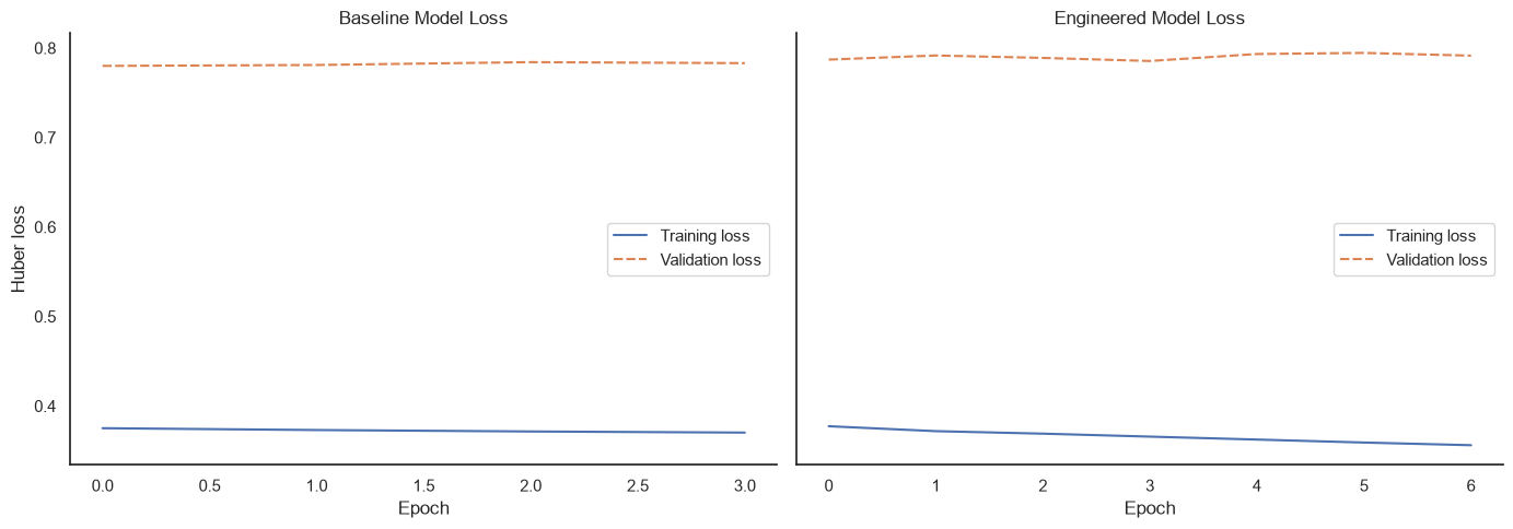

Training and validation loss for the baseline and the engineered feature set

Both runs stop early. The engineered model continues a few epochs longer, but a lower training loss would not by itself show that the extra inputs generalize. We need to compare predictions on the shared test period.

Step #6 Evaluate Model Performance

Feature engineering is inseparable from evaluation. We invert the scaled return predictions, reconstruct each next-session price from the previous observed Close, and compare both LSTMs with two naive strategies. Persistence predicts a zero return; median drift predicts the median Close return measured on training rows only.

baseline_scaled_predictions = baseline_model.predict(x_baseline_test, verbose=0)
engineered_scaled_predictions = engineered_model.predict(x_engineered_test, verbose=0)
baseline_return_predictions = target_scaler.inverse_transform(
  baseline_scaled_predictions
).ravel()
engineered_return_predictions = target_scaler.inverse_transform(
  engineered_scaled_predictions
).ravel()
actual_returns = target_scaler.inverse_transform(y_test.reshape(-1, 1)).ravel()

actual_prices = close_levels[test_target_indices]
previous_prices = close_levels[test_target_indices - 1]
median_training_return = float(np.median(close_returns[:train_size]))

predictions = {
  "Baseline LSTM": baseline_return_predictions,
  "Engineered LSTM": engineered_return_predictions,
  "Persistence": np.zeros_like(actual_returns),
  "Median drift": np.full_like(actual_returns, median_training_return),
}

metric_rows = []
predicted_prices = {}
for name, predicted_returns in predictions.items():
  prices = previous_prices * np.exp(predicted_returns)
  predicted_prices[name] = prices
  metric_rows.append(
    {
      "Model": name,
      "Price MAE": mean_absolute_error(actual_prices, prices),
      "Price RMSE": root_mean_squared_error(actual_prices, prices),
      "Return MAE (bps)": mean_absolute_error(
        actual_returns, predicted_returns
      ) * 10_000,
      "Directional accuracy (%)": np.mean(
        np.sign(actual_returns) == np.sign(predicted_returns)
      ) * 100,
    }
  )

metrics = pd.DataFrame(metric_rows).set_index("Model").round(2)
positive_return_rate = np.mean(actual_returns > 0) * 100
majority_class_accuracy = max(positive_return_rate, 100 - positive_return_rate)
print(f"Positive-return test sessions: {positive_return_rate:.1f}%")
print(f"Majority-class directional baseline: {majority_class_accuracy:.1f}%")
display(metrics)

results = pd.DataFrame(
  {"Actual": actual_prices, **predicted_prices},
  index=baseline_features.index[test_target_indices],
)
plot_results = results.loc["2024-01-01":]
_, axes = plt.subplots(nrows=2, ncols=1, figsize=(14, 10), sharex=True, sharey=True)
sns.lineplot(
  data=plot_results[["Actual", "Baseline LSTM", "Engineered LSTM"]],
  ax=axes[0],
)
axes[0].set_title("Feature-Set Comparison")
sns.lineplot(
  data=plot_results[["Actual", "Persistence", "Median drift"]],
  ax=axes[1],
)
axes[1].set_title("Naive Benchmarks")
for ax in axes:
  ax.set_ylabel(f"{stock_name} Close")
  ax.xaxis.set_major_locator(mdates.MonthLocator(interval=3))
  ax.xaxis.set_major_formatter(mdates.DateFormatter("%Y-%m"))

plt.tight_layout()
plt.show()

Positive-return test sessions: 56.7%
Majority-class directional baseline: 56.7%

                 Price MAE  Price RMSE  Return MAE (bps)  Directional accuracy (%)
Model
Baseline LSTM       148.49      213.04             91.80                     56.86
Engineered LSTM     149.08      213.85             92.18                     56.73
Persistence         150.85      213.73             93.14                      0.00
Median drift        149.28      213.29             92.27                     56.73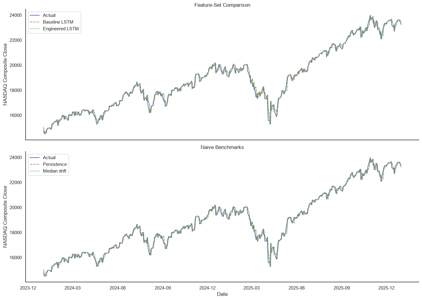

Feature-set comparison against the naive benchmarks on the held-out period

The baseline LSTM has the lowest price and return MAE, but its advantage is small: $0.59 over the engineered LSTM and$ 0.79 over median drift. The engineered inputs therefore do not improve this experiment.

Directional accuracy needs additional context. The test period rises on 56.7% of sessions, so a strategy that always predicts a positive return also scores 56.7%. The LSTMs remain at that same level. Persistence predicts no direction by definition, which is why its sign-based directional score is zero.

Step #7 Conclusions

Estimating which indicators will help in advance is difficult. Here, eight familiar technical indicators add model parameters and training epochs without improving out-of-sample error. The five-feature baseline records a $148.49 price MAE, compared with$ 149.08 for the engineered model, $149.28 for median drift, and$ 150.85 for persistence.

This result does not prove that technical indicators are always useless. It shows why feature engineering must be treated as a testable hypothesis. A credible comparison should:

calculate every feature using only information available at that timestamp;
fit preprocessing on training data only;
compare feature sets on identical target dates;
reserve chronological training data, rather than the test set, for model selection; and
include naive level and directional benchmarks.

Other feature definitions, architectures, assets, or market regimes may produce different results. Retain the extra complexity only when repeated out-of-sample tests show a useful and stable improvement.

Summary

In this tutorial, we created a causal 13-feature representation of NASDAQ market behavior from OHLCV changes, intraday range, moving-average distances, return volatility, Bollinger position, RSI, and MACD spread. We compared it with a five-feature OHLCV-change baseline using the same dates, model architecture, random seed, chronological split, and training-only preprocessing.

The simpler LSTM performed slightly better, and neither neural network showed a directional advantage over the test period’s positive-return frequency. That negative result is the main lesson: feature engineering is not the act of adding indicators, but the process of proposing, implementing, and honestly testing additional information.

The same workflow applies beyond financial data. Keep features causal, align candidate sets on common observations, isolate the test period, and compare every complex model with a sensible baseline.

And if you want to learn more about feature preparation and exploration, check out my recent article on Exploratory Feature Preparation for Regression Models.

Sources and Further Reading

The links above to Amazon are affiliate links. By buying through these links, you support the Relataly.com blog and help to cover the hosting costs. Using the links does not affect the price.

Books on Applied Machine Learning