Stock Market Forecasting Neural Networks for Multi-Output Regression in Python

Multi-output time series regression forecasts several future steps at once. In this tutorial, the final dense layer has ten neurons, with each neuron representing one future Apple close return. We reconstruct these returns into a ten-session price path. This direct multi-output approach avoids feeding predictions back into the model, although errors can still increase with the horizon.

We begin with the architecture of a multi-output neural network and then develop a compact Keras model. We transform prices and volume into daily log changes, fit preprocessing only on the training period, and create 50-input/10-output windows. After training with chronological validation, we reconstruct every held-out price path and compare it with a flat-price persistence baseline. Finally, we create an illustrative ten-session forecast.

Disclaimer

This article does not constitute financial advice. Stock markets can be very volatile and are generally difficult to predict. Predictive models and other forms of analytics applied in this article only serve the purpose of illustrating machine learning use cases.

Multi-Output Regression vs. Single-Output Regression

In time series regression, we train a statistical model on the past values of a time series to make statements about how the time series develops further. During model training, we feed the model with so-called mini-batches and the corresponding target values. The model then creates forecasts for all input batches and compares these predictions to the actual target values to calculate the residuals (prediction errors). In this way, the model can adjust its parameters iteratively and learn to make better predictions.

Multivariate forecasting models take into account multiple input variables, such as historical time series data and additional features like moving averages or momentum indicators, to improve the accuracy of their predictions. The idea is that these various variables can help the model identify patterns in the data that suggest future price movements.

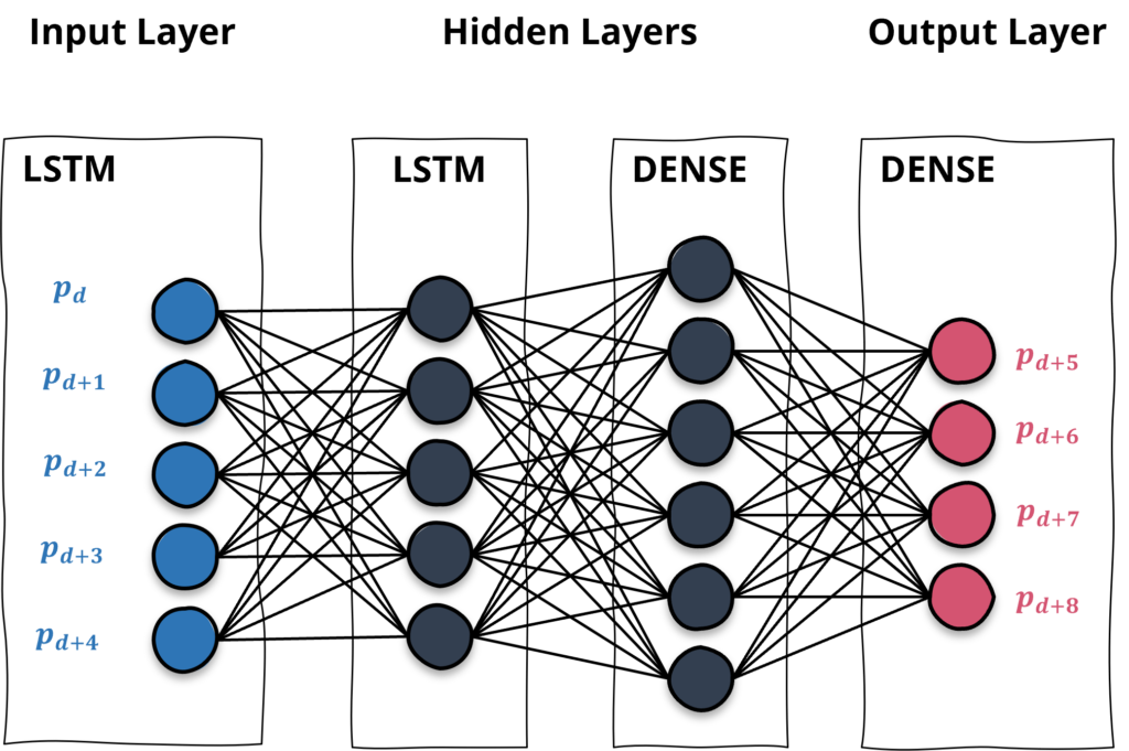
An exemplary architecture of a neural network with five input neurons (blue) and four output neurons (red)

The Architecture of a Neural Network with Multiple Outputs

Next, we will discuss the architecture of a neural network with multiple outputs. The input shape must match the sequence length and feature count. The number of hidden units is a model choice; it does not need to equal the number of input values. The number of output neurons determines the number of forecast horizons.

Models with a single neuron in the output layer are used to predict a single time step. It is possible to predict multiple price steps with a single-output model. It requires a rolling forecasting approach in which the outputs are iteratively reused to make further-reaching predictions. However, this way is somewhat cumbersome. A more elegant way is to train a multi-output model right away.

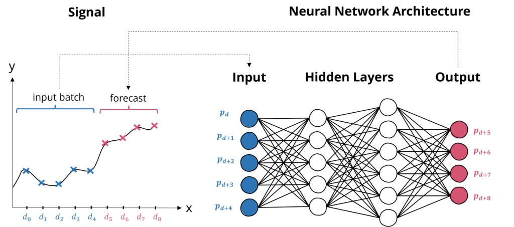
The inputs and outputs of a neural network for time series regression with five input neurons and four outputs

Training Neural Networks with Multiple Outputs

A model with multiple neurons in the output layer can predict numerous steps once per batch. Multi-output regression models train on many sequences of subsequent values, followed by the consecutive output sequence. The model architecture thus contains multiple neurons in the initial layer and various neurons in the output layer (as illustrated).

In a multi-output regression model, each output position is responsible for a different future horizon. To train such a model, you provide an input sequence followed by the corresponding output sequence. Here, 50 rows of five market-change features map to the next ten close returns.

The model will then learn to map the input sequence to the output sequence so that it can make predictions for multiple time steps in the future based on the input data.

In the next part of this tutorial, we will walk through the process of developing a multi-output regression model in more detail.

Implementing a Neural Network Model for Multi-Output Multi-Step Regression in Python

Let’s get started with the hands-on Python part. In the following, we will develop a neural network with Keras and Tensorflow that forecasts the Apple stock price. To prepare the data for a neural network with multiple outputs in time series forecasting, we will spend the most time preparing it and bringing it into the right shape. Broadly this involves the following steps:

1. Load the time series data that we want to use as input and output for your model. We use historical price data that is available via the yahoo finance API.
2. Transform price levels and volume into daily log changes.
3. Split chronologically, then fit preprocessing only on training rows.
4. Reshape the data and bring them into a format that can be input into the neural network. This involves converting the data into a 3D array for time series data.
5. Finally, we will train our model and generate the forecasting.

The code is available on the GitHub repository.

Neural network architectures with multiple outputs allow for more potent solutions but are more complex to train. Image created with Midjourney.

Prerequisites

Before beginning the coding part, ensure that you have set up your Python 3 environment and required packages. If you don’t have a Python environment, consider Anaconda. To set it up, you can follow the steps in this tutorial.

Also, make sure you install all required packages. In this tutorial, we will be working with the following standard packages:

• pandas
• NumPy
• matplotlib

In addition, we use Keras, scikit-learn, TensorFlow, seaborn, and yfinance. The refreshed notebook was tested with Python 3.12, TensorFlow 2.21, Keras 3.15, pandas 3.0, scikit-learn 1.9, and yfinance 1.5.

You can install these packages using console commands:

• pip install <package name>
• conda install <package name> (if you use the Anaconda package manager)

Step #1: Load the Data

We begin by loading adjusted historical Apple quotes with yfinance. A fixed endpoint keeps the train/test periods and reported metrics reproducible. Setting multi_level_index=False also keeps the single-ticker DataFrame shape explicit with current yfinance releases.

# Time Series Forecasting - Multi-output Regression for Stock Market Prediction
# A tutorial for this file is available at www.relataly.com
# Tested with Python 3.12, TensorFlow 2.21, Keras 3.15, pandas 3.0, and yfinance 1.5

import keras
import matplotlib.dates as mdates
import matplotlib.pyplot as plt
import numpy as np
import pandas as pd
import seaborn as sns
import tensorflow as tf
import yfinance as yf
from sklearn.metrics import mean_absolute_error, root_mean_squared_error
from sklearn.preprocessing import RobustScaler

sns.set_theme(style="white", rc={"axes.spines.right": False, "axes.spines.top": False})
keras.utils.set_random_seed(42)

print(f"TensorFlow version: {tf.__version__}")
print(f"Available GPUs: {len(tf.config.list_physical_devices('GPU'))}")

start_date = "2010-01-01"
end_date = "2026-01-01"
stock_name = "Apple"
symbol = "AAPL"

df = yf.download(
    symbol,
    start=start_date,
    end=end_date,
    auto_adjust=True,
    multi_level_index=False,
    progress=False,
)
if df.empty:
    raise RuntimeError("yfinance returned no data for AAPL")

print(df.shape)
df.head()

TensorFlow version: 2.21.0
Available GPUs: 0
(4024, 5)

The data should comprise the following columns:

• Close
• Open
• High
• Low
• Volume

With auto_adjust=True, the OHLC prices account for splits and dividends and no separate Adj Close column is returned. We will predict future close returns and reconstruct adjusted closing prices.

Step #2: Explore the Data

Once we have loaded the data, we print a quick overview of the time-series data using different line graphs. The following code will plot a line chart for each column in df_plot using the seaborn library. The charts will be organized in a grid with nrows number of rows and ncols number of columns. The sharex parameter is set to True, which means that the x-axes of the subplots will be shared. The figsize parameter determines the size of the plot in inches.

df_plot = df.copy()
_, axes = plt.subplots(nrows=3, ncols=2, sharex=True, figsize=(14, 9))

for ax, column in zip(axes.flat, df_plot.columns):
    sns.lineplot(x=df_plot.index, y=df_plot[column], ax=ax)
    ax.xaxis.set_major_locator(mdates.AutoDateLocator())
    ax.set_title(column)

for ax in axes.flat[len(df_plot.columns):]:
    ax.set_visible(False)

plt.tight_layout()
plt.show()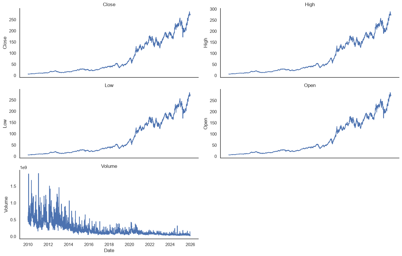

The line plots reflect Apple price and volume history through the fixed endpoint at the end of 2025.

Step #3: Preprocess the Data

Next, we prepare the data for the multi-output forecasting model. Preparing data for multivariate forecasting involves several steps:

• Transforming the market series into features that are more stationary than price levels
• Splitting the observations chronologically
• Fitting all preprocessing on the training period only
• Slicing the time series into overlapping input and output sequences

These choices are specific to this example. Other time series can require different transformations, features, and validation designs.

3.1 Basic Preparations

We begin by sorting the dates and removing incomplete rows. Keeping the DatetimeIndex makes later forecast plots easier to interpret.

df_train = df.sort_index().dropna().copy()
df_train.tail()

3.2 Feature Selection and Scaling

Stock prices are non-stationary levels: their scale changes substantially over a long sample, and a model trained directly on those levels can learn the historical range instead of transferable price movements. We therefore calculate one-session log returns for Open, High, Low, and Close, plus the log change in Volume. The model’s ten targets are future Close log returns.

We retain separate RobustScaler instances for the five inputs and the one target. Most importantly, both scalers are fit on training rows only. Transforming later rows with those fitted scalers is valid; fitting on the whole series would leak the center and spread of the test period into training. I have covered feature engineering in a separate article if you want to explore further transformations.

price_columns = ["Open", "High", "Low", "Close"]
price_log_returns = np.log(df_train[price_columns]).diff()
volume_log_change = np.log1p(df_train["Volume"]).diff().rename("Volume")
features = pd.concat([price_log_returns, volume_log_change], axis=1).dropna()

feature_values = features.to_numpy()
close_returns = features[["Close"]].to_numpy()
close_levels = df_train.loc[features.index, "Close"].to_numpy()
train_size = int(len(features) * 0.8)

feature_scaler = RobustScaler()
feature_scaler.fit(feature_values[:train_size])
scaled_features = feature_scaler.transform(feature_values)

target_scaler = RobustScaler()
target_scaler.fit(close_returns[:train_size])
scaled_close_returns = target_scaler.transform(close_returns)

print(f"Features: {features.columns.tolist()}")
print(f"Transformed shape: {features.shape}")
print(f"Training rows: {train_size}")

Features: ['Open', 'High', 'Low', 'Close', 'Volume']
Transformed shape: (4023, 5)
Training rows: 3218

The final step of the data preparation is to create the structure for the input data. This structure needs to match the input layer of the model architecture.

3.3 Slicing the Data for a Model with Multiple In- and Outputs

The sliding-window function maps 50 rows of five input features to the ten Close returns immediately following them. It also records where each target path starts. We use that position to create strict train and test masks: every training target ends before the split, while the first test target starts at the split. Historical rows before the boundary remain available as context for the first test sample.

input_sequence_length = 50
output_sequence_length = 10


def create_multi_output_sequences(
    feature_values,
    target_values,
    input_sequence_length,
    output_sequence_length,
):
    inputs, targets, target_starts = [], [], []
    final_start = len(feature_values) - output_sequence_length + 1
    for target_start in range(input_sequence_length, final_start):
        inputs.append(feature_values[target_start - input_sequence_length:target_start])
        targets.append(target_values[target_start:target_start + output_sequence_length, 0])
        target_starts.append(target_start)

    return (
        np.asarray(inputs, dtype=np.float32),
        np.asarray(targets, dtype=np.float32),
        np.asarray(target_starts),
    )


x_all, y_all, target_starts = create_multi_output_sequences(
    scaled_features,
    scaled_close_returns,
    input_sequence_length,
    output_sequence_length,
)
train_mask = target_starts + output_sequence_length - 1 < train_size
test_mask = target_starts >= train_size

x_train, y_train = x_all[train_mask], y_all[train_mask]
x_test, y_test = x_all[test_mask], y_all[test_mask]
test_target_starts = target_starts[test_mask]

print(f"Training shapes: {x_train.shape}, {y_train.shape}")
print(f"Test shapes: {x_test.shape}, {y_test.shape}")

assert target_starts[train_mask][-1] + output_sequence_length - 1 < train_size
assert test_target_starts[0] == train_size
print(
    "First test path:",
    features.index[test_target_starts[0]].date(),
    "->",
    features.index[test_target_starts[0] + output_sequence_length - 1].date(),
)

Training shapes: (3159, 50, 5), (3159, 10)
Test shapes: (796, 50, 5), (796, 10)
First test path: 2022-10-17 -> 2022-10-28

Step #4: Prepare the Neural Network Architecture and Train the Multi-Output Regression Model

Now that the training data is ready, the next step is to configure the multi-output neural network. Because each input sequence contains five features, this is also a multivariate architecture.

4.1 Configuring and Training the Model

We use a compact architecture: an LSTM with 32 units, a 32-unit dense layer, and ten linear outputs. The explicit Input layer follows the current Keras 3 API. Huber loss behaves quadratically for small residuals and linearly for larger ones, making training less sensitive to unusually large return observations than mean squared error.

model = keras.Sequential(
    [
        keras.layers.Input(shape=(input_sequence_length, x_train.shape[2])),
        keras.layers.LSTM(32),
        keras.layers.Dense(32, activation="relu"),
        keras.layers.Dense(output_sequence_length),
    ],
    name="apple_multi_output_lstm",
)
model.compile(
    optimizer=keras.optimizers.Adam(),
    loss=keras.losses.Huber(),
)
model.summary()

The final 10% of the training sequences provides chronological validation. The test period remains untouched until final evaluation. We disable shuffling, monitor validation loss, and restore the weights from the best epoch.

early_stopping = keras.callbacks.EarlyStopping(
    monitor="val_loss",
    patience=3,
    restore_best_weights=True,
)
history = model.fit(
    x_train,
    y_train,
    batch_size=32,
    epochs=20,
    validation_split=0.1,
    shuffle=False,
    callbacks=[early_stopping],
    verbose=1,
)

4.2 Loss Curve

Next, we plot training and validation loss. Falling training loss alone does not establish predictive performance; the validation curve is what early stopping monitors while tuning the weights.

loss_history = pd.DataFrame(
    {
        "Training loss": history.history["loss"],
        "Validation loss": history.history["val_loss"],
    }
)

_, ax = plt.subplots(figsize=(10, 5))
sns.lineplot(data=loss_history, ax=ax)
ax.set_title("Model Loss")
ax.set_xlabel("Epoch")
ax.set_ylabel("Huber loss")
plt.show()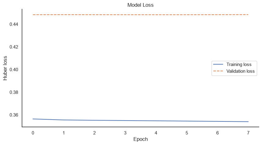

The curves show optimization progress on scaled returns. We still need to reconstruct prices and compare the model with a simple out-of-sample benchmark before judging its usefulness.

Step #5 Evaluate Model Performance

Now that we have trained the model, we can finally use the test set. The network predicts scaled log returns, so we first invert the target scaling. Cumulative sums turn each return sequence into cumulative log returns, and exponentiation reconstructs prices from the close immediately before each forecast begins.

We compare these reconstructed paths with persistence, which assumes the last observed close remains unchanged throughout the ten-session horizon. This is a difficult baseline to beat for daily stock prices and gives the neural network’s errors essential context. We report aggregate MAE and RMSE across all 7,960 held-out price points, along with MAE at each horizon.

predicted_returns_scaled = model.predict(x_test, verbose=0)
predicted_returns = target_scaler.inverse_transform(
    predicted_returns_scaled.reshape(-1, 1)
).reshape(-1, output_sequence_length)
actual_returns = target_scaler.inverse_transform(
    y_test.reshape(-1, 1)
).reshape(-1, output_sequence_length)

origin_indices = test_target_starts - 1
origin_prices = close_levels[origin_indices]
predicted_prices = origin_prices[:, np.newaxis] * np.exp(
    np.cumsum(predicted_returns, axis=1)
)
actual_prices = origin_prices[:, np.newaxis] * np.exp(
    np.cumsum(actual_returns, axis=1)
)
persistence_prices = np.repeat(
    origin_prices[:, np.newaxis],
    output_sequence_length,
    axis=1,
)

model_mae = mean_absolute_error(actual_prices.ravel(), predicted_prices.ravel())
model_rmse = root_mean_squared_error(actual_prices.ravel(), predicted_prices.ravel())
baseline_mae = mean_absolute_error(actual_prices.ravel(), persistence_prices.ravel())
baseline_rmse = root_mean_squared_error(actual_prices.ravel(), persistence_prices.ravel())

horizon_metrics = pd.DataFrame(
    {
        "Horizon": np.arange(1, output_sequence_length + 1),
        "LSTM MAE": [
            mean_absolute_error(actual_prices[:, horizon], predicted_prices[:, horizon])
            for horizon in range(output_sequence_length)
        ],
        "Persistence MAE": [
            mean_absolute_error(actual_prices[:, horizon], persistence_prices[:, horizon])
            for horizon in range(output_sequence_length)
        ],
    }
)

print(f"LSTM path MAE: ${model_mae:.2f}")
print(f"LSTM path RMSE: ${model_rmse:.2f}")
print(f"Persistence path MAE: ${baseline_mae:.2f}")
print(f"Persistence path RMSE: ${baseline_rmse:.2f}")
print(horizon_metrics.round(2).to_string(index=False))

sample_number = 50
sample_start = test_target_starts[sample_number]
history_slice = slice(sample_start - input_sequence_length, sample_start)
future_slice = slice(sample_start, sample_start + output_sequence_length)

_, ax = plt.subplots(figsize=(16, 6))
sns.lineplot(
    x=features.index[history_slice],
    y=close_levels[history_slice],
    ax=ax,
    label="Observed",
)
sns.lineplot(
    x=features.index[future_slice],
    y=actual_prices[sample_number],
    ax=ax,
    color="black",
    marker="o",
    label="Actual future",
)
sns.lineplot(
    x=features.index[future_slice],
    y=predicted_prices[sample_number],
    ax=ax,
    color="#C92A2A",
    marker="o",
    label="LSTM forecast",
)
sns.lineplot(
    x=features.index[future_slice],
    y=persistence_prices[sample_number],
    ax=ax,
    color="#2B8A3E",
    linestyle=":",
    label="Persistence",
)
ax.set_title("Ten-Session Multi-Output Forecast Example")
ax.set_ylabel("Adjusted Apple close (USD)")
plt.show()

LSTM path MAE: $5.57
LSTM path RMSE: $7.80
Persistence path MAE: $5.62
Persistence path RMSE: $7.79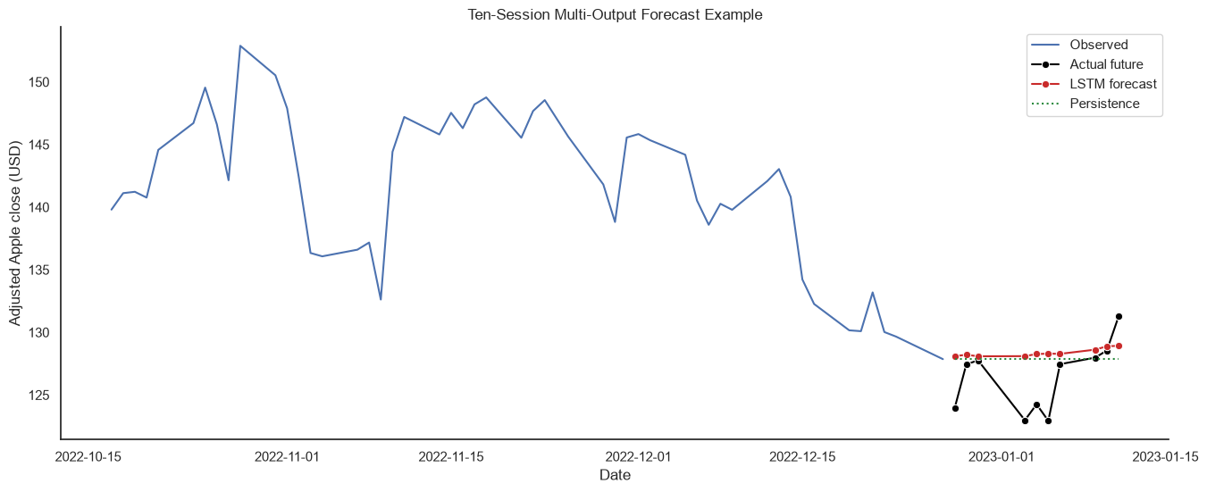

The LSTM’s MAE is only $0.05 lower than persistence, while its RMSE is$0.01 higher. This difference is too small and inconsistent to claim a meaningful forecasting advantage. The useful result here is the end-to-end multi-output method, not evidence that this feature set can predict Apple profitably. A stronger experiment would repeat training across random seeds and market regimes, compare additional baselines, and include trading costs before drawing practical conclusions.

Step #6 Create a New Forecast

Finally, we pass the latest 50 transformed observations to the model, invert the ten predicted returns, and reconstruct a price path from the last observed adjusted close. We label the x-axis by trading-session horizon instead of inventing future dates without an exchange calendar. The result is illustrative: it is a conditional model output, not a recommendation or a demonstrated edge.

latest_input = scaled_features[-input_sequence_length:].reshape(
    1,
    input_sequence_length,
    scaled_features.shape[1],
)
future_returns_scaled = model.predict(latest_input, verbose=0)
future_returns = target_scaler.inverse_transform(
    future_returns_scaled.reshape(-1, 1)
).ravel()

last_close = float(close_levels[-1])
future_prices = last_close * np.exp(np.cumsum(future_returns))
future_forecast = pd.DataFrame(
    {
        "Horizon": np.arange(1, output_sequence_length + 1),
        "LSTM forecast": future_prices,
        "Persistence": last_close,
    }
)

print(f"Last observed adjusted close on {features.index[-1].date()}: ${last_close:.2f}")
print(future_forecast.round(2).to_string(index=False))

history_positions = np.arange(-input_sequence_length + 1, 1)
future_positions = future_forecast["Horizon"].to_numpy()

_, ax = plt.subplots(figsize=(14, 5))
sns.lineplot(
    x=history_positions,
    y=close_levels[-input_sequence_length:],
    ax=ax,
    label="Observed",
)
sns.lineplot(
    x=future_positions,
    y=future_forecast["LSTM forecast"],
    ax=ax,
    color="#C92A2A",
    marker="o",
    label="Illustrative LSTM forecast",
)
sns.lineplot(
    x=future_positions,
    y=future_forecast["Persistence"],
    ax=ax,
    color="#2B8A3E",
    linestyle=":",
    label="Persistence",
)
ax.axvline(0, color="gray", linewidth=1)
ax.set_title("Illustrative Ten-Session Apple Forecast")
ax.set_xlabel("Trading sessions relative to the latest observation")
ax.set_ylabel("Adjusted close (USD)")
plt.show()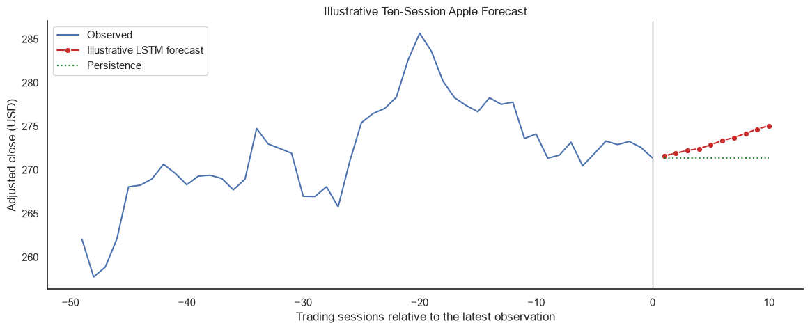

In this seeded run, the illustrative path reaches approximately $275.06 at horizon ten. That number can vary with training randomness and should be interpreted alongside the baseline result above.

Summary

In this tutorial, we built a direct multi-output LSTM that maps 50 sessions of five Apple market-change features to ten future Close returns. We fitted preprocessing only on the training period, reserved chronological training data for validation, kept the test period out of model selection, and reconstructed adjusted price paths for evaluation.

The comparison is as important as the architecture. The LSTM achieved a path MAE of $5.57 versus$5.62 for persistence, but its RMSE was $7.80 versus$7.79. It therefore showed no meaningful advantage on this test period. This is a realistic result for daily stock returns and a reminder that a technically correct forecast pipeline does not guarantee useful predictive signal.

You can extend the experiment with other stationary features, architectures, seeds, and walk-forward evaluation. Changing the output length requires rebuilding the target windows and output layer, followed by fresh out-of-sample evaluation. Any claimed improvement should consistently beat simple baselines rather than only produce a plausible-looking chart.

I hope this article was helpful in understanding multi-output neural networks better. If you have any questions or comments, please let me know.

Sources and Further Reading

1. Charu C. Aggarwal (2018) Neural Networks and Deep Learning
2. Jansen (2020) Machine Learning for Algorithmic Trading: Predictive models to extract signals from market and alternative data for systematic trading strategies with Python
3. Aurélien Géron (2019) Hands-On Machine Learning with Scikit-Learn, Keras, and TensorFlow: Concepts, Tools, and Techniques to Build Intelligent Systems
4. David Forsyth (2019) Applied Machine Learning Springer
5. Andriy Burkov (2020) Machine Learning Engineering

The links above to Amazon are affiliate links. By buying through these links, you support the Relataly.com blog and help to cover the hosting costs. Using the links does not affect the price.

If you want to learn about an alternative approach to univariate stock market forecasting, consider taking a look at Facebook Prophet or ARIMA models