Measuring Regression Errors with Python

Evaluating performance is a crucial step in developing regression models. Because regression models return continuous outputs, such models allow for different gradations of right or wrong. Therefore, we measure the deviation between predictions and actual values in numerical terms. However, a universal metric to measure the performance of regression models does not exist. Instead, there are several metrics, each with its advantages and disadvantages. None of these metrics is sufficient alone, and it is often necessary to use them in combination. This article presents six regression error metrics and explains how to implement them in Python with Scikit-learn.

The rest of this article proceeds in two parts. The first part is conceptual and introduces six error metrics for measuring regression performance. We look at formulas and discuss their pros and cons. The discussion is summarized in a cheat sheet. The second part is a hands-on Python tutorial in which we generate synthetic time series data and use them for training a prediction model. Then we implement the six regression error metrics and evaluate the performance of our model.

Note that this article deals with regression errors. If you are looking for an overview of classification error metrics, check out this tutorial on classification error metrics.

goal arrow shot archery machine learning error metrics

Measuring Regression Errors

In general, we measure the performance of regression models by calculating the deviations between the predictions (y_pred) and the actual values (y_test). If the prediction value is below the actual value, the prediction error is positive. If the prediction lies above the real value, the prediction error is negative. However, in a sample of prediction values, the errors can vary greatly depending on the data point. Therefore, it is not enough to look at individual error values. Error metrics can inform us about the statistical distribution of errors in a prediction sample and, in this way, help us to measure the performance of regression models objectively.

Various metrics exist to measure regression errors. Each error metric can only cover a part of the overall picture. For instance, imagine you have developed a model to predict the consumption of a power plant. The model predictions are generally accurate, but the projections are wrong in a few cases. In other words, outliers among the prediction errors make it difficult to conclude the model performance. It is insufficient to calculate the average prediction error to understand this situation. Instead, a more robust measuring approach would combine different error metrics to conclude the probability that prediction errors lie within a specific range.

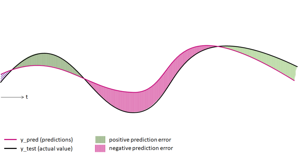
Predictions vs. Actual Values in Time Series Forecasting

Six Error Metrics for Measuring Regression Errors

The following six metrics help measure prediction errors. We can apply them to various regression problems, including time series forecasting.

• Mean Absolute Error (MAE)
• Mean Absolute Percentage Error (MAPE)
• Median Absolute Error (MedAE)
• Mean Squared Error (MSE)
• Root Mean Squared Error (RMSE)
• Median Absolute Percent Error (MdAPE)

Mean Absolute Error (MAE)

Mean Absolute Error (MAE) is a metric commonly used to measure the arithmetic average of deviations between predictions and actual values.

An MAE of “5” tells us that, on average, our predictions deviate from the actual values by 5. Whether this error is considered small or large will depend on the application case and the scale of the predictions. For instance, 5 nanometers in the case of a building might be small, but if it’s five nanometers in the case of a biological membrane, it might be significant. So when working with the MAE, mind the scale.

• It is scale-dependent
• The MAE uses absolute values so positive and negative residuals do not cancel each other out.
• The MAE is less sensitive to outliers than squared-error metrics, but large errors can still affect its mean.
• The MAE shares the same unit with the predictions.

Mean Absolute Percentage Error (MAPE)

The mean absolute percentage error calculates the mean percentage deviation between predictions and actual values.

• The MAPE is scale-independent, which can make comparisons across differently scaled positive targets easier.
• MAPE is undefined when an actual value is zero and unstable when actual values are close to zero.
• Percentage interpretation is problematic when the target can be negative, as in the synthetic series below.

Mean Squared Error (MSE)

We can calculate the MSE by measuring the average squares of the differences between the estimated and actual values.

• Since all values are squared, the MSE is very sensitive to outliers.
• MSE is expressed in squared target units, so its numerical value should not be compared directly with MAE. Use RMSE when you want squared-error sensitivity in the original unit. The formula of the MSE is:

Median Absolute Error (MedAE)

The Median Absolute Error (MedAE) calculates the median deviation between predictions and actual values.

• The MedAE has the same unit as the predictions.
• A MedAE of 10 means that half of the absolute errors are at most 10 and half are at least 10.
• The MedAE is resistant to outliers. We often use it with the MAE; a large gap between them indicates that a minority of large errors is pulling up the mean.

Root Mean Squared Error (RMSE)

The root-mean-squared error is another standard way to measure the performance of a forecasting model.

• It has the same unit as the target and predictions.
• Squaring emphasizes larger errors before the square root restores the original unit.
• RMSE is not robust to outliers.

Median Absolute Percentage Error (MdAPE)

The median absolute percentage error (MdAPE) is similar to MAPE but calculates the median percentage error for a set of forecasts. As a result, MdAPE is more resistant to a minority of extreme ratios than MAPE. A MdAPE of 5% means that half of the absolute percentage errors are at most 5%, and half are at least 5%.

• Scale-independent.
• Undefined when an actual value is zero and unstable near zero.
• More resistant to a minority of extreme percentage errors than MAPE, but the median does not fix the zero-denominator problem.

Implementing Regression Error Metrics in Python: Time Series Prediction Example

Now that we have familiarized ourselves with standard regression error metrics, it’s time to see them in action. In the following, we will develop and test a regression model in Python. We begin by generating synthetic time series data. Subsequently, we use the data to train a simple regression model based on a Keras neural network. The model will try to continue the time series and predict a continuous value for the next time step. We will use this model to predict a test dataset and measure prediction performance with the error metrics.

The code of this Python example is available on the GitHub repository.

Prerequisites

Before starting the coding part, make sure you have set up a Python 3 environment. This version was tested with Python 3.12, TensorFlow 2.21, Keras 3.15, NumPy 2.5, pandas 3.0, and scikit-learn 1.9. The project repository contains the complete dependency list.

Step #1 Generate Synthetic Time Series Data

We begin by generating synthetic time series data. The script below creates the time series by multiplying different sine curves.

# Measuring Regression Model Performance
# A tutorial for this file is available at www.relataly.com
# Tested with Python 3.12, TensorFlow 2.21, Keras 3.15, NumPy 2.5, and scikit-learn 1.9

import keras
import matplotlib.pyplot as plt
import numpy as np
import pandas as pd
import seaborn as sns
from sklearn.metrics import (
  mean_absolute_error,
  mean_absolute_percentage_error,
  mean_squared_error,
  median_absolute_error,
  root_mean_squared_error,
)
from sklearn.preprocessing import StandardScaler

sns.set_theme(style="white", rc={"axes.spines.right": False, "axes.spines.top": False})
keras.utils.set_random_seed(42)

steps = np.arange(1_000)
values = (
  100
  * np.sin(np.pi * steps * 0.02 + 0.01)
  * np.sin(np.pi * steps * 0.005 + 0.01) ** 2
)
df = pd.DataFrame({"Value": values}, index=pd.Index(steps, name="Step"))

near_zero_count = int((df["Value"].abs() < 1).sum())
print(f"Value range: {df['Value'].min():.2f} to {df['Value'].max():.2f}")
print(f"Targets with |actual| < 1: {near_zero_count}")

fig, ax = plt.subplots(figsize=(14, 4))
sns.lineplot(data=df, x=df.index, y="Value", ax=ax)
ax.set_title("Synthetic Time Series")
plt.tight_layout()
plt.show()

Value range: -87.40 to 86.48
Targets with |actual| < 1: 105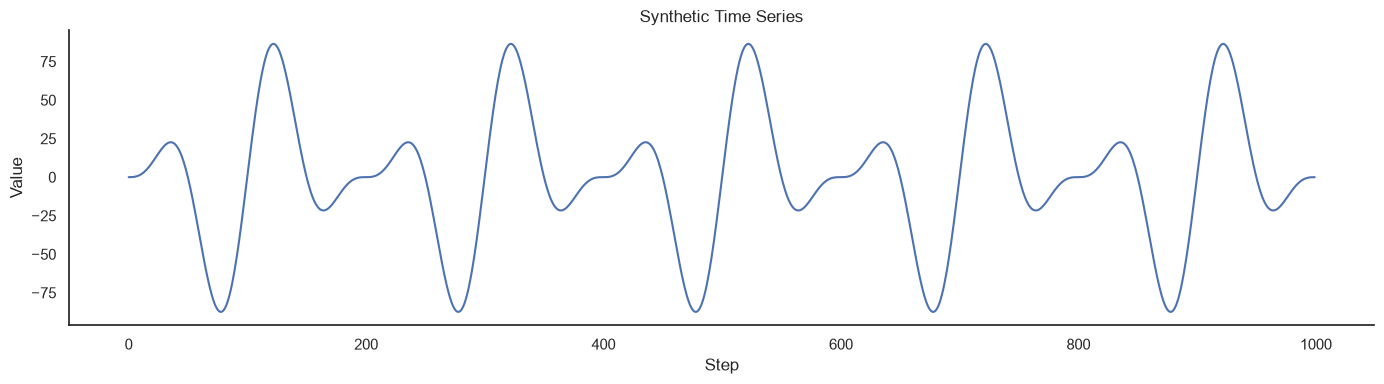

Step #2 Data Preparation

Now that we have the synthetic data available, we can prepare it as input for our regression model. We choose the chronological 80% training boundary before fitting StandardScaler, so the test period cannot influence preprocessing. Each sample contains 15 values and predicts the following value.

values_2d = df[["Value"]].to_numpy()
train_size = int(len(values_2d) * 0.8)
sequence_length = 15

scaler = StandardScaler()
scaler.fit(values_2d[:train_size])
scaled_values = scaler.transform(values_2d)


def create_sequences(data, sequence_length):
  inputs, targets, target_indices = [], [], []
  for target_index in range(sequence_length, len(data)):
    inputs.append(data[target_index - sequence_length:target_index])
    targets.append(data[target_index, 0])
    target_indices.append(target_index)

  return (
    np.asarray(inputs, dtype=np.float32),
    np.asarray(targets, dtype=np.float32),
    np.asarray(target_indices),
  )


x_all, y_all, target_indices = create_sequences(scaled_values, sequence_length)
train_mask = target_indices < train_size
test_mask = target_indices >= train_size

x_train, y_train = x_all[train_mask], y_all[train_mask]
x_test, y_test = x_all[test_mask], y_all[test_mask]
test_target_indices = target_indices[test_mask]

print(f"Training sequences: {x_train.shape}, targets: {y_train.shape}")
print(f"Test sequences: {x_test.shape}, targets: {y_test.shape}")
assert test_target_indices[0] == train_size
print(
  f"First test target: step {test_target_indices[0]} "
  f"using data through step {test_target_indices[0] - 1}"
)

Training sequences: (785, 15, 1), targets: (785,)
Test sequences: (200, 15, 1), targets: (200,)
First test target: step 800 using data through step 799

Step #3 Training a Time Series Regression Model

Once we have prepared the data, we can train the regression model. The compact network uses one 16-unit LSTM and a linear output. We keep the latest 10% of training windows for chronological validation, preserve sequence order, and restore the weights with the lowest validation loss. The test set remains untouched.

keras.utils.set_random_seed(42)
model = keras.Sequential(
  [
    keras.layers.Input(shape=(sequence_length, 1)),
    keras.layers.LSTM(16),
    keras.layers.Dense(1),
  ],
  name="synthetic_series_lstm",
)
model.compile(
  optimizer=keras.optimizers.Adam(),
  loss="mean_squared_error",
)
early_stopping = keras.callbacks.EarlyStopping(
  monitor="val_loss",
  patience=5,
  restore_best_weights=True,
)
history = model.fit(
  x_train,
  y_train,
  batch_size=32,
  epochs=50,
  validation_split=0.1,
  shuffle=False,
  callbacks=[early_stopping],
  verbose=0,
)

print(f"Parameters: {model.count_params():,}")
print(f"Epochs trained: {len(history.history['loss'])}")
print(f"Best validation MSE: {min(history.history['val_loss']):.5f}")

loss_history = pd.DataFrame(
  {
    "Training loss": history.history["loss"],
    "Validation loss": history.history["val_loss"],
  }
)
sns.lineplot(data=loss_history)
plt.xlabel("Epoch")
plt.ylabel("Mean squared error")
plt.title("Training History")
plt.tight_layout()
plt.show()

Parameters: 1,169
Epochs trained: 50
Best validation MSE: 0.00283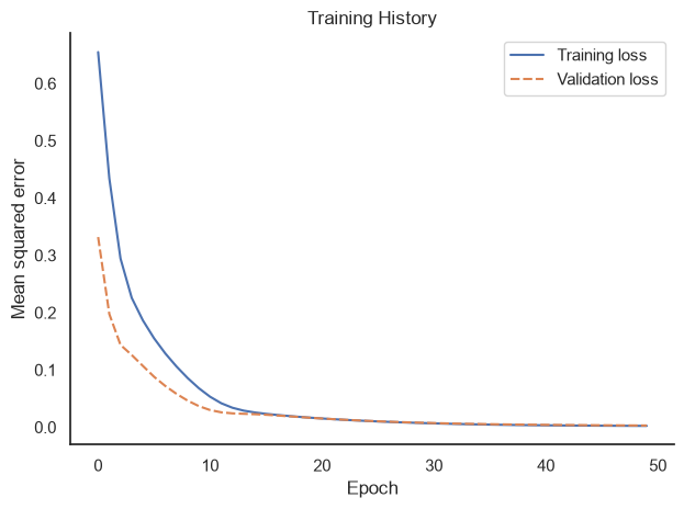

Step #4 Making Test Predictions

Let’s see how the model performs on the test set. We inverse-transform its predictions and add a persistence baseline that predicts the last observed value. A metric is much easier to interpret when we know whether a simple rule achieves a similar result.

scaled_predictions = model.predict(x_test, verbose=0)
y_pred = scaler.inverse_transform(scaled_predictions).ravel()
y_test_unscaled = scaler.inverse_transform(y_test.reshape(-1, 1)).ravel()
y_persistence = values_2d[test_target_indices - 1, 0]

print(f"Predictions: {y_pred.shape}")
print(f"Actual values: {y_test_unscaled.shape}")
print(f"Persistence baseline: {y_persistence.shape}")

Predictions: (200,)
Actual values: (200,)
Persistence baseline: (200,)

Next, we plot the predictions and signed residuals, defined as actual minus predicted. Residuals above zero indicate underprediction; residuals below zero indicate overprediction.

test_df = pd.DataFrame(
  {
    "Actual": y_test_unscaled,
    "LSTM": y_pred,
    "Persistence": y_persistence,
  },
  index=pd.Index(test_target_indices, name="Step"),
)
residuals = pd.DataFrame(
  {
    "LSTM residual": y_test_unscaled - y_pred,
    "Persistence residual": y_test_unscaled - y_persistence,
  },
  index=test_df.index,
)

fig, axes = plt.subplots(
  nrows=2,
  ncols=1,
  figsize=(14, 8),
  sharex=True,
  gridspec_kw={"height_ratios": [2, 1]},
)
sns.lineplot(data=test_df, ax=axes[0])
axes[0].set_title("One-Step Predictions")
axes[0].set_ylabel("Value")

sns.lineplot(data=residuals, ax=axes[1])
axes[1].axhline(0, color="black", linewidth=1)
axes[1].set_title("Signed Residuals (Actual - Prediction)")
axes[1].set_ylabel("Residual")

plt.tight_layout()
plt.show()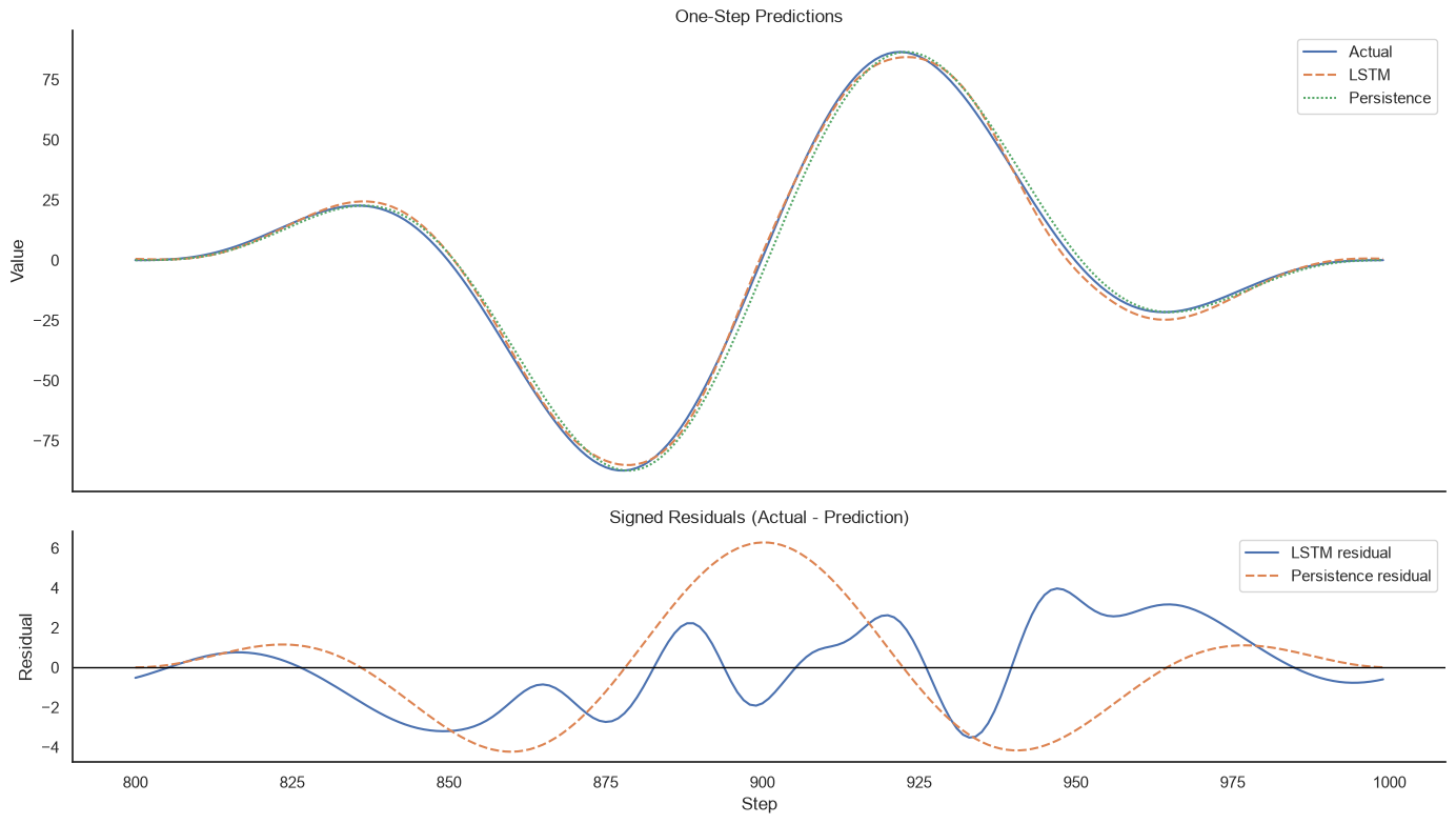

The plot shows that the prediction errors vary and are sometimes positive and sometimes negative.

Step #5 Calculating the Regression Error Metrics: Implementation and Evaluation

Now that we have predicted the test set, we calculate all six metrics for the LSTM and persistence. In practice, use the subset that matches the target domain and the cost of errors; reporting more numbers does not repair an unsuitable metric.

def median_absolute_percentage_error(actual, predicted):
  with np.errstate(divide="ignore", invalid="ignore"):
    absolute_percentage_errors = np.abs((actual - predicted) / actual)
  return float(np.median(absolute_percentage_errors) * 100)


def regression_metrics(actual, predicted):
  return {
    "MAE": mean_absolute_error(actual, predicted),
    "MedAE": median_absolute_error(actual, predicted),
    "MSE": mean_squared_error(actual, predicted),
    "RMSE": root_mean_squared_error(actual, predicted),
    "MAPE (%)": mean_absolute_percentage_error(actual, predicted) * 100,
    "MdAPE (%)": median_absolute_percentage_error(actual, predicted),
  }


metrics = pd.DataFrame(
  {
    "LSTM": regression_metrics(y_test_unscaled, y_pred),
    "Persistence": regression_metrics(y_test_unscaled, y_persistence),
  }
).T

near_zero_test_count = int((np.abs(y_test_unscaled) < 1).sum())
print(metrics.round(2).to_string())
print(f"\nTest targets with |actual| < 1: {near_zero_test_count} of {len(y_test_unscaled)}")
print("MAPE and MdAPE are not reliable for this zero-crossing target.")

        MAE  MedAE   MSE  RMSE  MAPE (%)  MdAPE (%)
LSTM         1.65   1.53  3.90  1.97   4529.80       7.48
Persistence  2.18   1.47  8.02  2.83     45.25       9.46

Test targets with |actual| < 1: 21 of 200
MAPE and MdAPE are not reliable for this zero-crossing target.

Step #6 Interpreting the Regression Error Metrics

Start with the scale-dependent metrics. The LSTM improves MAE from 2.18 to 1.65 and RMSE from 2.83 to 1.97 compared with persistence. It therefore reduces both average absolute error and the larger misses emphasized by squared error. MSE communicates the same squared-error objective, but its unit is value squared; RMSE is easier to interpret on the original scale.

MedAE tells a different story. Persistence scores 1.47, slightly better than the LSTM’s 1.53. This means the LSTM reduces average and larger errors without improving the median absolute error. The ranking difference is exactly why we use multiple metrics and a baseline.

The percentage metrics are not valid rankings for this target. The series crosses zero, includes negative values, and has 21 of 200 test targets with an absolute magnitude below 1. Dividing by those tiny actual values inflates the LSTM’s MAPE to 4529.80%, even though the LSTM has lower MAE and RMSE than persistence. MdAPE is less affected by a minority of extreme ratios, but it does not fix the zero or near-zero denominator and should not be used here either.

Summary

This article presented six regression error metrics and demonstrated them on a synthetic time series. We fitted preprocessing on training data only, trained a compact LSTM with chronological validation, and compared it with persistence on an untouched test period.

Different metrics answer different questions. MAE summarizes average absolute error, MedAE describes the typical absolute error robustly, and RMSE emphasizes larger misses while remaining in the target unit. MSE carries the same ranking as RMSE but is expressed in squared units. MAPE and MdAPE can be useful for strictly positive targets bounded away from zero; they are unsuitable for this zero-crossing series.

Choose metrics from the target domain and the cost of mistakes, inspect residuals, and always include a simple baseline. A metric table is useful only when every value is mathematically meaningful for the data being evaluated.

I hope this article was helpful. If you have any remarks or questions remaining, write them in the comments.