Rolling Time Series Forecasting: Creating a Multi-Step Prediction for a Rising Sine Curve using Neural Networks in Python

Many time series forecasting problems can be solved by predicting just one step into the future. However, some problems require a forecast over an extended horizon. In this article, we use a rising sine curve to demonstrate recursive multi-step forecasting with a Keras LSTM model. The model predicts the next change, appends that prediction to its input history, and repeats the process for 30 steps.

The remainder of this article proceeds as follows: We begin with the sine curve problem and a quick introduction to recurrent neural networks. We then generate synthetic data, model first differences rather than the rising level, and train a compact univariate LSTM. Finally, we evaluate both one-step predictions and the complete 30-step rollout against persistence. Because the future is generated by a known function, we can measure recursive forecast error directly.

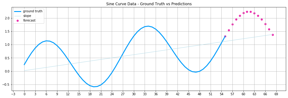
A multi-step time series forecast for a rising sine curve, as we will create in this article.

If you are just getting started with time-series forecasting, we have covered the single-step forecasting approach in two previous articles:

Predicting Stock Markets with Neural Networks - A Step-by-Step Guide Stock Market Prediction – Adjusting Time Series Prediction Intervals in Python

The Problem of a Rising Sine Curve

The line plot below illustrates the sample of a rising sine curve. The goal is to use the ground truth values (blue) to forecast several points in this curve (purple).

The signal in this tutorial is fully deterministic, so using its generating formula would be simpler and exact. The LSTM is intentionally an educational example: it lets us observe how a learned one-step model behaves when its predictions become future inputs. Real signals are usually noisier, less regular, and harder to forecast.

Also: Stock Market Prediction using Univariate Recurrent Neural Networks (RNN) with Python

Application Domains with Similar Time Series Forecasting Problems

A rising sine wave may sound like an abstract problem at first. However, similar issues are widespread. Imagine you are the owner of an online shop. The users who visit your shop and buy something fluctuate depending on the time and the weekday. For instance, there are fewer visitors at night, and on weekends, the number of visitors rises sharply. At the same time, the overall number of users increases over a more extended period as the shop becomes known to a broader audience. To plan the number of goods to be held in stock, you need to see the number of orders at any point in time over several weeks. It is a typical multi-step time series problem, and similar problems exist in various domains:

• Healthcare: e.g., forecasting of health signals such as heart, blood, or breathing signals
• Network Security: e.g., analysis of network traffic in intrusion detection systems
• Sales and Marketing: e.g., forecasting of market demand
• Production demand forecasting: e.g., for power consumption and capacity planning
• Prediction and filtering of sensor signals, e.g., of audio signals

A time series forecasting problem: predicting sine curve data

Recurrent Neural Networks for Time Series Forecasting

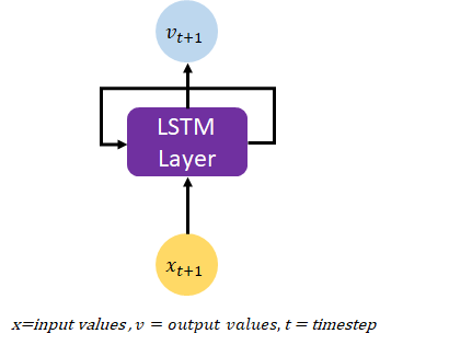
The model used in this article is a recurrent neural network with a Long Short-Term Memory (LSTM) layer. Unlike a feedforward layer, an LSTM updates hidden and cell states while processing the time steps within each input sequence. That state helps it represent temporal dependencies. The recursive loop in this tutorial is separate inference logic: after training, our Python code appends each predicted change to the next input window.

Also: Mastering Multivariate Stock Market Prediction with Python: A Guide to Effective Feature Engineering Techniques

The Training Process of a Recurrent Neural Network

When training neural networks, the process typically involves multiple epochs, where an epoch refers to a single pass through the entire training dataset. During each epoch, the neural network receives the entire training data and adjusts its weights accordingly through forward and backward propagation. The batch size, which determines the number of examples passed through the network at once, also affects how the weights are updated between neurons.

It’s important to note that one epoch is usually not enough for the model to learn the underlying patterns and relationships in the data, leading to underfitting and poor performance in prediction tasks. Hence, multiple epochs are often needed to fine-tune the network and improve its predictive capabilities. However, care must be taken not to overfit the model by choosing too many epochs. Overfitting occurs when the model becomes too complex and performs well on the training data but poorly on any other data, resulting in poor generalization.

To avoid overfitting, we can employ various techniques such as early stopping, where the training process is stopped when the validation loss begins to increase, indicating that the model is overfitting. Another method is to use regularization techniques such as L1 or L2 regularization, dropout, or data augmentation to prevent overfitting and improve the model’s generalization capabilities.

Functioning of an LSTM layer

An LSTM (Long Short-Term Memory) layer is a specialized type of recurrent neural network (RNN) layer that is specifically designed for processing and making predictions based on time series data. Unlike traditional RNNs, which suffer from the vanishing gradient problem, LSTM layers can maintain a memory of past events and selectively use this memory to make predictions about future events.

LSTM layers accomplish this by incorporating several unique mechanisms, such as gates and cell states. The gates control the flow of information into and out of the cell, while the cell state represents the memory of the network. These mechanisms work together to enable LSTM layers to learn and make predictions based on long-term dependencies in the data, which is a characteristic of many time series datasets.

An LSTM does not automatically generate an arbitrary number of future steps. Our model produces one next-step change. To create a recursive forecast, we repeatedly call the trained model and reuse each output as part of the following input. This is simple and flexible, but errors can accumulate as the forecast moves further from observed data.

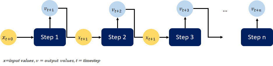
Functioning of an LSTM layer

LSTM Components

To understand how an LSTM layer works, it is helpful to think about the layer as consisting of several different components, each of which has a specific role in the overall operation of the layer. These components include the following:

1. Input gate: The input gate controls which information from the input data will be passed on to the cell state. The input gate uses a sigmoid activation function to determine which information should be retained and which should be discarded.
2. Forget gate: The forget gate controls which information from the cell state will be discarded. The forget gate uses a sigmoid activation function to determine which information should be forgotten and which should be retained.
3. Cell state: The cell state is a vector that contains the information that is retained by the LSTM layer. This information is updated at each time step based on the input from the input gate and the forget gate.
4. Output gate: The output gate controls which information from the cell state will be passed on to the output of the LSTM layer. The output gate uses a sigmoid activation function to determine which information should be retained and which should be discarded.

This article uses LSTM layers combined with a rolling forecast approach to predict the course of a sinus curve with a linear slope. The result is a multi-step time series forecast.

Creating a Rolling Multi-Step Time Series Forecast in Python

In this tutorial, we will explore the process of creating a rolling multi-step forecast using Python. Our dataset for this exercise will be a synthetically generated rising sine curve, which we will use to demonstrate the principles of multi-step time series forecasting.

By following the steps outlined in this tutorial, you will see how chronological splitting, differencing, leakage-free scaling, baseline comparison, and recursive evaluation fit together.

To get started, we have made the code available on our GitHub repository. You can easily access and follow along with the tutorial by downloading the code and running it on your local machine. This will enable you to experiment with different parameters and modify the code to suit your specific requirements.

Prerequisites

Before starting the coding part, make sure that you have set up your Python 3 environment and required packages. If you don’t have an environment yet, you can follow this tutorial to set up the Anaconda environment.

Also, make sure you install all required packages. In this tutorial, we will be working with the following standard packages:

• pandas
• NumPy
• matplotlib

In addition, we use Keras with the TensorFlow backend, seaborn, and scikit-learn. The refreshed notebook was tested with Python 3.12, TensorFlow 2.21, Keras 3.15, pandas 3.0, and scikit-learn 1.9.

You can install packages using console commands:

• pip install <package name>
• conda install <package name> (if you use the Anaconda package manager)

Step #1 Generating Synthetic Data

We begin by loading the required packages and creating a synthetic dataset. The synthetic data contains 300 values of the sinus function combined with a slight linear upward slope of 0.02. The code below creates the data and visualizes it in a line plot.

# A tutorial for this file is available at www.relataly.com
# Tested with Python 3.12, TensorFlow 2.21, Keras 3.15, pandas 3.0, and scikit-learn 1.9

import keras
import matplotlib.pyplot as plt
import numpy as np
import pandas as pd
import seaborn as sns
import tensorflow as tf
from sklearn.metrics import mean_absolute_error, root_mean_squared_error
from sklearn.preprocessing import RobustScaler

sns.set_theme(style="white", rc={"axes.spines.right": False, "axes.spines.top": False})
keras.utils.set_random_seed(42)

print(f"TensorFlow version: {tf.__version__}")
print(f"Available GPUs: {len(tf.config.list_physical_devices('GPU'))}")


def generate_signal(indices, gradient=0.02, frequency=0.125):
    indices = np.asarray(indices, dtype=np.float32)
    return gradient * indices + np.sin(np.pi * frequency * indices)


n_observations = 300
time_index = np.arange(n_observations)
df = pd.DataFrame({"sine_curve": generate_signal(time_index)}, index=time_index)

_, ax = plt.subplots(figsize=(16, 4))
sns.lineplot(data=df, ax=ax, color="#167D9A")
ax.set_title("Synthetic Trend and Sine Wave")
ax.set_xlabel("Time step")
ax.set_ylabel("Value")
plt.show()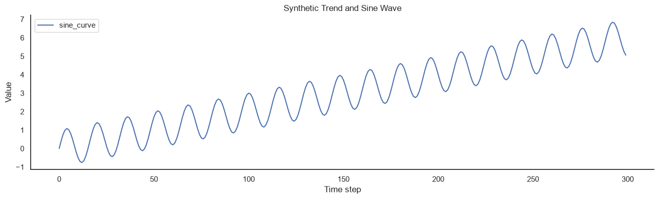

The signal curve oscillates and is steadily moving upward.

Step #2 Preprocessing

Next, we preprocess the data for the neural network. Running the code below will perform the following tasks:

• Split the 300 observations chronologically into 240 training and 60 test values.
• Convert the rising level to first differences. The repeating changes are easier for the model to learn and can be accumulated back into forecast levels.
• Fit RobustScaler only on training changes so the held-out period cannot influence preprocessing.
• Create 32-step input windows, covering two complete periods of the sine component.

Also: Mastering Multivariate Stock Market Prediction with Python: A Guide to Effective Feature Engineering Techniques

values = df[["sine_curve"]].to_numpy()
train_size = int(len(values) * 0.8)
changes = np.diff(values, axis=0)
train_change_count = train_size - 1

# Model changes rather than the trending level, and fit preprocessing on training changes only.
scaler = RobustScaler()
scaler.fit(changes[:train_change_count])
scaled_changes = scaler.transform(changes)

print(f"Training observations: {train_size}")
print(f"Test observations: {len(values) - train_size}")

sequence_length = 32


def create_sequences(series, sequence_length):
    features, targets = [], []
    for target_index in range(sequence_length, len(series)):
        features.append(series[target_index - sequence_length:target_index])
        targets.append(series[target_index, 0])

    return (
        np.asarray(features, dtype=np.float32),
        np.asarray(targets, dtype=np.float32),
    )


train_changes = scaled_changes[:train_change_count]
test_changes = scaled_changes[train_change_count - sequence_length:]
x_train, y_train = create_sequences(train_changes, sequence_length)
x_test, y_test = create_sequences(test_changes, sequence_length)
test_index = df.index[train_size:]

print(f"Training shapes: {x_train.shape}, {y_train.shape}")
print(f"Test shapes: {x_test.shape}, {y_test.shape}")

assert np.isclose(x_test[0, -1, 0], scaled_changes[train_change_count - 1, 0])
assert np.isclose(y_test[0], scaled_changes[train_change_count, 0])

Training observations: 240
Test observations: 60
Training shapes: (207, 32, 1), (207,)
Test shapes: (60, 32, 1), (60,)

Step #3 Build and Train the One-Step Model

Now that we have prepared the synthetic data, we define a compact neural network. The input layer accepts 32 scaled changes. The LSTM summarizes this sequence, and the dense layers produce the next scaled change.

3.1 Overview of Model Parameters

Finding the optimal configuration is often a process of trial and error. Below you find a list of model parameters with which you can experiment:

Keras model parameters used in this tutorial epoch: An epoch is an iteration over the entire x_train and y_train data provided. Batch_size: Number of samples per gradient update. If unspecified, batch_size is 32. Activation: Mathematical equations determine whether a neuron in the network should activate (“fired”) or not. Input_shape: Tensor with shape: (batch_size, …, input_dim). Input_len: the length of the generated input sequence. Return_sequences: If set to false, the layer will return the final output in the output sequence. If true, the layer returns the entire series. Loss: The loss function tells the model how to evaluate its performance so that the weights can be updated to reduce the loss on the following evaluation. Optimizer: Every time a neural network finishes processing a batch through the network and generates prediction results, the optimizer decides how to adjust weights between the nodes.

Source: keras.io/layers/recurrent - view the Keras documentation for a complete list of parameters.

3.2 Choosing Model Parameters

Finding a suitable architecture still requires systematic experiments. Here, the model is deliberately small: 32 LSTM units and a 16-unit dense layer are enough for this deterministic pattern. The sequence length does not need to equal the number of LSTM units.

model = keras.Sequential(
    [
        keras.layers.Input(shape=(sequence_length, 1)),
        keras.layers.LSTM(32),
        keras.layers.Dense(16, activation="relu"),
        keras.layers.Dense(1),
    ],
    name="recursive_sine_forecaster",
)
model.compile(optimizer=keras.optimizers.Adam(), loss="mean_squared_error")

epochs = 100
batch_size = 16
early_stopping = keras.callbacks.EarlyStopping(
    monitor="val_loss",
    patience=10,
    restore_best_weights=True,
)
history = model.fit(
    x_train,
    y_train,
    batch_size=batch_size,
    epochs=epochs,
    validation_split=0.2,
    shuffle=False,
    callbacks=[early_stopping],
    verbose=0,
)

best_epoch = int(np.argmin(history.history["val_loss"]) + 1)
print(f"Stopped after {len(history.history['loss'])} epochs")
print(f"Best validation epoch: {best_epoch}")

Stopped after 100 epochs
Best validation epoch: 100

The exact stopping epoch can vary slightly across TensorFlow builds and hardware. The callback restores the best validation weights whether training stops early or reaches the 100-epoch maximum.

Step #4 Predicting a Single-step Ahead

We continue by predicting each held-out next change using only observed input values. We invert the scaling, add each predicted change to its forecast origin, and compare the reconstructed levels with both the ground truth and persistence. Persistence assumes no change from the latest observation.

predicted_changes_scaled = model.predict(x_test, verbose=0)
predicted_changes = scaler.inverse_transform(predicted_changes_scaled).ravel()
actual_changes = scaler.inverse_transform(y_test.reshape(-1, 1)).ravel()

forecast_origins = df["sine_curve"].iloc[train_size - 1:-1].to_numpy()
y_pred = forecast_origins + predicted_changes
y_test_unscaled = df["sine_curve"].iloc[train_size:].to_numpy()

absolute_percentage_errors = np.abs((y_test_unscaled - y_pred) / y_test_unscaled) * 100
mae = mean_absolute_error(y_test_unscaled, y_pred)
rmse = root_mean_squared_error(y_test_unscaled, y_pred)
mape = absolute_percentage_errors.mean()

# Persistence predicts no change from the latest observed value.
naive_pred = forecast_origins
naive_mae = mean_absolute_error(y_test_unscaled, naive_pred)
naive_rmse = root_mean_squared_error(y_test_unscaled, naive_pred)

print(f"LSTM one-step MAE: {mae:.4f}")
print(f"LSTM one-step RMSE: {rmse:.4f}")
print(f"LSTM one-step MAPE: {mape:.3f}%")
print(f"Persistence MAE: {naive_mae:.4f}")
print(f"Persistence RMSE: {naive_rmse:.4f}")

LSTM one-step MAE: 0.0010
LSTM one-step RMSE: 0.0013
LSTM one-step MAPE: 0.021%
Persistence MAE: 0.2544
Persistence RMSE: 0.2802

The differenced LSTM clearly beats persistence on this synthetic held-out period. That establishes that the one-step model has learned the repeating change pattern before we expose it to the harder recursive task.

Step #5 Visualizing Predictions and Loss

Next, we plot the held-out one-step predictions together with the ground truth and persistence baseline.

one_step_results = pd.DataFrame(
    {
        "Actual": y_test_unscaled,
        "LSTM": y_pred,
        "Persistence": naive_pred,
    },
    index=test_index,
)

_, ax = plt.subplots(figsize=(16, 5))
sns.lineplot(data=one_step_results, ax=ax)
ax.set_title("Held-Out One-Step Predictions")
ax.set_xlabel("Time step")
ax.set_ylabel("Value")
plt.show()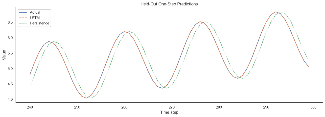

The LSTM line closely follows the actual values, while persistence visibly lags around turning points. We also inspect training and validation loss. The dashed marker shows the epoch whose weights are retained.

loss_history = pd.DataFrame(
    {
        "Training loss": history.history["loss"],
        "Validation loss": history.history["val_loss"],
    }
)

_, ax = plt.subplots(figsize=(10, 5))
sns.lineplot(data=loss_history, ax=ax)
ax.axvline(best_epoch - 1, color="#C92A2A", linestyle="--", label="Best epoch")
ax.set_title("Model Loss")
ax.set_xlabel("Epoch")
ax.set_ylabel("Mean squared error")
ax.legend()
plt.show()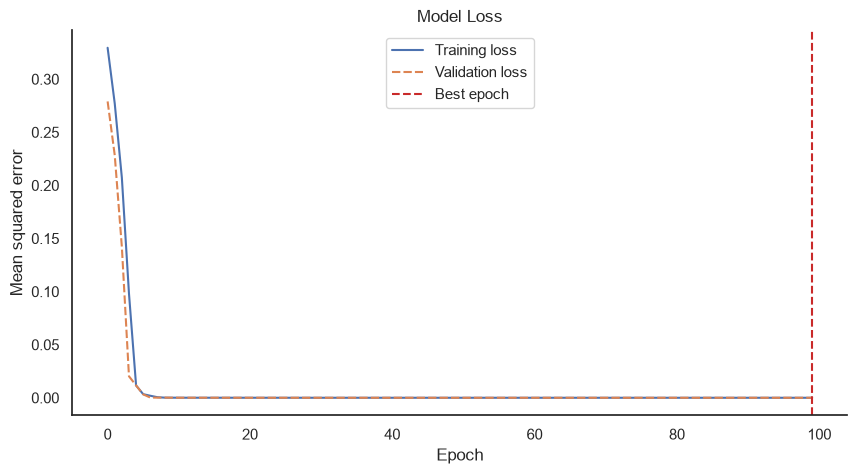

Step #6 Rolling Forecasting: Creating a Multi-step Time Series Forecast

Next, we generate the recursive multi-step forecast. We initialize the process with the final 32 observed changes. Each predicted change is appended to that list and becomes part of the next model input. We then invert the scaling and cumulatively add the predicted changes to the final observed level.

Recursive errors can compound, so evaluating only the one-step model is not enough. The signal generator gives us the actual 30 future values, allowing a direct rollout comparison.

Also: Measuring Regression Errors with Python

The forecasting process begins with an initial prediction for a single time step. After that, we add the predicted value to the input values for another projection, and so on. In this way, we create the rolling forecast with multiple time steps.

forecast_steps = 30
rolling_scaled_changes = scaled_changes[-sequence_length:, 0].astype(np.float32).tolist()
forecast_changes_scaled = []

for _ in range(forecast_steps):
    x_input = np.asarray(
        rolling_scaled_changes[-sequence_length:],
        dtype=np.float32,
    ).reshape(1, sequence_length, 1)
    next_change_scaled = float(model.predict(x_input, verbose=0)[0, 0])
    forecast_changes_scaled.append(next_change_scaled)
    rolling_scaled_changes.append(next_change_scaled)

forecast_changes = scaler.inverse_transform(
    np.asarray(forecast_changes_scaled).reshape(-1, 1)
).ravel()
forecast_index = np.arange(n_observations, n_observations + forecast_steps)
forecast_values = float(values[-1, 0]) + np.cumsum(forecast_changes)
actual_future = generate_signal(forecast_index)
persistence_forecast = np.repeat(float(values[-1, 0]), forecast_steps)

rollout_mae = mean_absolute_error(actual_future, forecast_values)
rollout_rmse = root_mean_squared_error(actual_future, forecast_values)
persistence_rollout_mae = mean_absolute_error(actual_future, persistence_forecast)
persistence_rollout_rmse = root_mean_squared_error(actual_future, persistence_forecast)

forecast = pd.DataFrame(
    {
        "Actual future": actual_future,
        "Recursive LSTM": forecast_values,
        "Persistence": persistence_forecast,
    },
    index=forecast_index,
)

print(f"Recursive {forecast_steps}-step MAE: {rollout_mae:.4f}")
print(f"Recursive {forecast_steps}-step RMSE: {rollout_rmse:.4f}")
print(f"Persistence {forecast_steps}-step MAE: {persistence_rollout_mae:.4f}")
print(f"Persistence {forecast_steps}-step RMSE: {persistence_rollout_rmse:.4f}")

Recursive 30-step MAE: 0.0010
Recursive 30-step RMSE: 0.0013
Persistence 30-step MAE: 1.2920
Persistence 30-step RMSE: 1.4937

The recursive LSTM remains close to the known future across all 30 steps and substantially outperforms constant persistence. We can now plot the observed history, actual future, and both forecasts together.

history_window = df.iloc[-100:]

_, ax = plt.subplots(figsize=(16, 5))
sns.lineplot(
    x=history_window.index,
    y=history_window["sine_curve"],
    ax=ax,
    label="Observed",
)
sns.lineplot(
    x=forecast.index,
    y=forecast["Actual future"],
    ax=ax,
    color="black",
    linestyle="--",
    label="Actual future",
)
sns.lineplot(
    x=forecast.index,
    y=forecast["Recursive LSTM"],
    ax=ax,
    color="#C92A2A",
    marker="o",
    label="Recursive LSTM",
)
sns.lineplot(
    x=forecast.index,
    y=forecast["Persistence"],
    ax=ax,
    color="#2B8A3E",
    linestyle=":",
    label="Persistence",
)
ax.axvline(n_observations - 1, color="gray", linewidth=1)
ax.set_title("Thirty-Step Recursive Forecast")
ax.set_xlabel("Time step")
ax.set_ylabel("Value")
plt.show()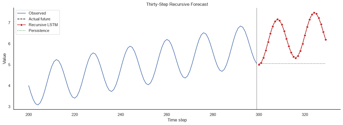

Step #7 Interpreting the Result

The differenced representation is the decisive improvement. A model trained directly on rising levels must extrapolate beyond the range used to fit its scaler and network weights. Changes remain within the repeating range represented in training, and accumulating them restores the trend.

This nearly exact result should not be generalized to real data. The synthetic future follows the same deterministic formula as the training period and contains no noise, regime changes, missing observations, or external shocks. For real recursive forecasts, use walk-forward evaluation across multiple origins and inspect how error changes with each horizon.

Summary

In this tutorial, we created a recursive 30-step forecast for a rising sine curve. We fitted preprocessing only on training data, modeled first differences, validated the one-step model against persistence, and measured the complete rollout against the known future.

The main lesson is not that an LSTM is necessary for a sine wave. It is that recursive forecasting must be evaluated as a recursive process: strong one-step accuracy does not guarantee a strong multi-step rollout. The representation also matters. Modeling changes allowed this compact network to learn a stable repeating pattern without extrapolating raw levels beyond the training range.

For real time series, broaden the evaluation to several forecast origins and compare with seasonal persistence or domain-specific baselines. Direct and multi-output models are useful alternatives when recursive error accumulation becomes too large.

I hope this article was helpful. If you have questions remaining, let me know in the comments.

Another forecasting approach is to train a neural network model that predicts multiple outputs per input batch. Another relataly article demonstrates how this multi-output regression approach works: Stock Market Prediction - Multi-output regression in Python.

Also, consider non-neural network approaches to time series forecasting, such as ARIMA, which can achieve great results too.

Sources and Further Reading

The links above to Amazon are affiliate links. By buying through these links, you support the Relataly.com blog and help to cover the hosting costs. Using the links does not affect the price.