Geographic Choropleth Maps with GeoPandas and Python

A choropleth map colors geographic areas according to a numeric value. This tutorial uses GeoPandas to join country-level COVID-19 records to Natural Earth boundaries, create a world map, and zoom in on Africa and Europe.

The workflow is reproducible: it uses an archived Johns Hopkins snapshot from December 31, 2022 instead of a moving “latest day.” Missing countries remain gray, values are normalized by population, and every map states when its color scale is capped.

The complete executed notebook is available in the Relataly Python tutorials repository.

Choropleth Maps and Geographic Heat Maps

A choropleth assigns a color to each polygon, such as a country or administrative region. Darker or more saturated colors usually indicate larger values. The technique works well for rates, percentages, and other normalized measures tied to defined areas.

The term “geographic heat map” is often used more broadly. A true heat map may estimate continuous density from point locations, while a choropleth preserves polygon boundaries. The maps in this tutorial are choropleths.

Common pitfalls include:

• Mapping raw counts when populations differ substantially.
• Treating missing observations as zero.
• Allowing one extreme value to flatten the remaining color range.
• Using a rainbow palette whose visual order is ambiguous.
• Comparing maps with different units, periods, or color scales.
• Forgetting that large geographic areas attract more visual attention.

We address these issues with per-capita metrics, explicit missing-data colors, sequential palettes, ranked tables, and documented percentile capping.

Prerequisites

Install the required packages with:

pip install pandas matplotlib geopandas country-converter

The executed notebook uses Python 3.12, GeoPandas 1.1, and pandas 3.0.

Step 1: Load a Fixed COVID-19 Snapshot

The original tutorial used a retired statworx endpoint and selected “yesterday,” which no longer produced a reproducible result. The revised version uses the archived Johns Hopkins global confirmed-case time series.

We compare November 30 and December 31, 2022 to calculate newly reported cases during December. Cruise ships and sporting-event records are excluded because they are not countries.

import country_converter as coco
import geopandas as gpd
import matplotlib.pyplot as plt
import pandas as pd

COVID_URL = (
    "https://raw.githubusercontent.com/CSSEGISandData/COVID-19/master/"
    "csse_covid_19_data/csse_covid_19_time_series/"
    "time_series_covid19_confirmed_global.csv"
)
SNAPSHOT_COLUMN = "12/31/22"
PERIOD_START_COLUMN = "11/30/22"
NON_COUNTRY_ROWS = {
    "Diamond Princess",
    "MS Zaandam",
    "Summer Olympics 2020",
    "Winter Olympics 2022",
}

confirmed_raw = pd.read_csv(COVID_URL)
country_cases = (
    confirmed_raw.loc[~confirmed_raw["Country/Region"].isin(NON_COUNTRY_ROWS)]
    .groupby("Country/Region", as_index=False)[
        [PERIOD_START_COLUMN, SNAPSHOT_COLUMN]
    ]
    .sum()
    .rename(
        columns={
            PERIOD_START_COLUMN: "period_start_cases",
            SNAPSHOT_COLUMN: "total_cases",
        }
    )
)
country_cases["new_cases_december"] = (
    country_cases["total_cases"] - country_cases["period_start_cases"]
).clip(lower=0)
country_cases["iso3"] = coco.convert(
    names=country_cases["Country/Region"],
    to="ISO3",
    not_found=None,
)
country_cases = country_cases.loc[country_cases["iso3"].str.len() == 3]

The executed result contains 197 country records. The United States, India, France, Germany, and Brazil have the largest cumulative confirmed totals in this snapshot.

Step 2: Load Natural Earth Boundaries

GeoPandas reads the Natural Earth GeoJSON file directly. We retain the country name, ISO-3 code, continent, population estimate, and geometry.

BOUNDARIES_URL = (
    "https://raw.githubusercontent.com/nvkelso/natural-earth-vector/master/"
    "geojson/ne_110m_admin_0_countries.geojson"
)

boundaries = gpd.read_file(BOUNDARIES_URL)[
    ["ADMIN", "ADM0_A3", "CONTINENT", "POP_EST", "geometry"]
]
boundaries = boundaries.rename(
    columns={
        "ADMIN": "country",
        "ADM0_A3": "iso3",
        "CONTINENT": "continent",
        "POP_EST": "population_estimate",
    }
)
boundaries = boundaries.loc[boundaries["country"] != "Antarctica"].copy()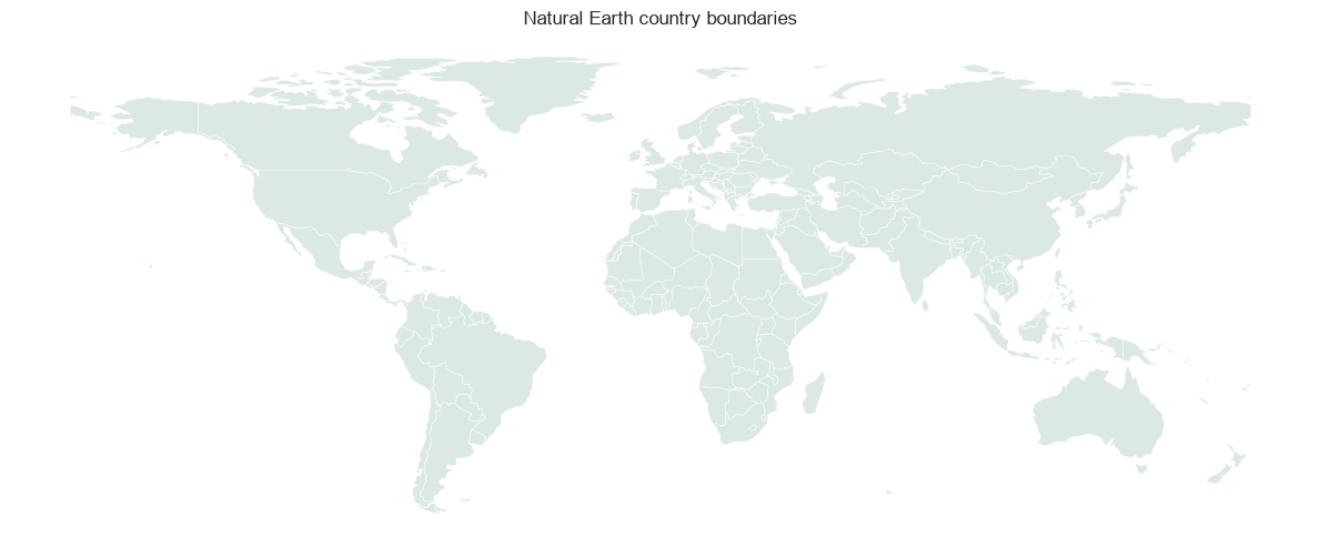

The geometry table is the left side of the join. This choice preserves countries that lack a matched COVID record, allowing the map to render those areas as missing.

Step 3: Join and Normalize the Data

ISO-3 codes provide a more reliable join key than country names. The executed join matches COVID data to 93.2% of the map geometries. Twelve geometries remain unmatched, including territories and disputed or differently represented areas.

world = boundaries.merge(
    country_cases,
    on="iso3",
    how="left",
    validate="one_to_one",
)
world["cases_per_100k"] = (
    world["total_cases"] / world["population_estimate"] * 100_000
)
world["new_cases_december_per_100k"] = (
    world["new_cases_december"] / world["population_estimate"] * 100_000
)

match_rate = world["total_cases"].notna().mean()
assert world.geometry.notna().all()
assert match_rate > 0.9

Natural Earth population values are estimates, so the rates are approximate. They are still more comparable across countries than raw counts.

Step 4: Build a Reusable Choropleth Function

The plotting helper caps values at the 98th percentile for color assignment. The underlying data remains unchanged. This keeps extreme observations from consuming most of the color range.

def plot_choropleth(frame, column, title, colorbar_label, cmap="YlOrRd"):
    values = frame[column].dropna()
    upper_limit = values.quantile(0.98)
    normalized_values = frame[column].clip(upper=upper_limit)

    fig, ax = plt.subplots(figsize=(12, 6))
    frame.assign(plot_value=normalized_values).plot(
        column="plot_value",
        ax=ax,
        cmap=cmap,
        edgecolor="white",
        linewidth=0.35,
        legend=True,
        legend_kwds={"label": colorbar_label, "shrink": 0.65},
        missing_kwds={"color": "#d9d9d9", "label": "No matched data"},
    )
    ax.set_title(title, fontsize=16, pad=12)
    ax.axis("off")
    fig.tight_layout()
    return fig, ax

Step 5: Map December 2022 Cases Worldwide

The world map shows newly reported confirmed cases during December 2022 per 100,000 residents.

world_figure, world_axis = plot_choropleth(
    world,
    column="new_cases_december_per_100k",
    title="Reported COVID-19 cases during December 2022",
    colorbar_label=(
        "New confirmed cases per 100,000 (capped at 98th percentile)"
    ),
)

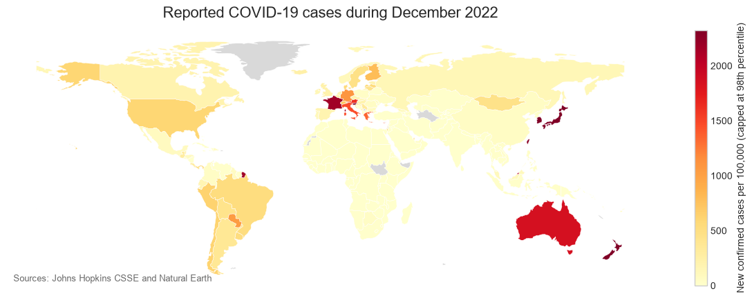
South Korea and Japan have the highest mapped December rates, at approximately 3,792 and 3,500 newly reported cases per 100,000. New Zealand, Slovenia, and Taiwan follow. These figures describe reported cases and should not be read as infection prevalence.

Step 6: Zoom In on Africa

Filtering a GeoDataFrame uses the same syntax as filtering a pandas DataFrame. The Africa map shows cumulative confirmed cases per 100,000 through December 31, 2022.

africa = world.loc[world["continent"] == "Africa"].copy()

africa_figure, africa_axis = plot_choropleth(
    africa,
    column="cases_per_100k",
    title="Cumulative confirmed COVID-19 cases in Africa through 2022",
    colorbar_label=(
        "Confirmed cases per 100,000 (capped at 98th percentile)"
    ),
    cmap="YlGnBu",
)

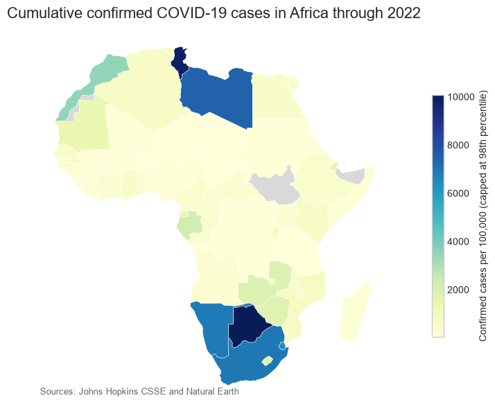
Botswana has the largest mapped cumulative rate in Africa at about 14,232 confirmed cases per 100,000, followed by Tunisia, Libya, South Africa, and Namibia. Differences in testing and reporting capacity are especially important when comparing these totals.

Step 7: Zoom In on Europe

The Europe map returns to the December-incidence metric. Explicit longitude and latitude limits prevent Russia’s full extent from compressing central and western Europe.

europe = world.loc[world["continent"] == "Europe"].copy()

europe_figure, europe_axis = plot_choropleth(
    europe,
    column="new_cases_december_per_100k",
    title="Reported COVID-19 cases in Europe during December 2022",
    colorbar_label=(
        "New confirmed cases per 100,000 (capped at 98th percentile)"
    ),
    cmap="PuBuGn",
)
europe_axis.set_xlim(-25, 45)
europe_axis.set_ylim(34, 72)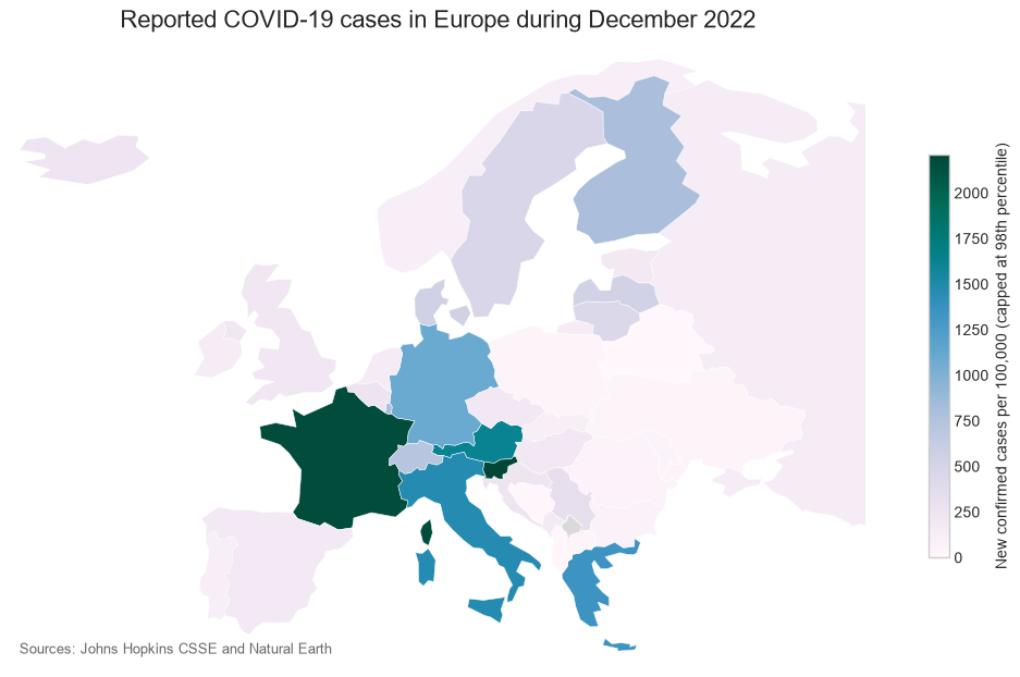

Slovenia and France have the largest mapped European December rates, at approximately 2,347 and 2,165 cases per 100,000. Austria, Italy, and Greece complete the top five.

Interpretation and Limitations

These maps describe confirmed cases in an archived reporting system. They do not measure every infection. Testing access, case definitions, reporting delays, revisions, and national surveillance practices differ. Population denominators are estimates, and unmatched geometries remain gray.

Choropleths also emphasize land area. A large, sparsely populated country occupies more visual space than a small, densely populated country with the same rate. Pairing each map with a ranked table prevents area from becoming a proxy for importance.

For a production analysis, use matching population estimates for the observation year, document territorial handling, and test sensitivity to different clipping thresholds. Use a shared color range when visual comparisons between separate maps are the primary goal.

Summary

This tutorial built reproducible choropleth maps with GeoPandas by combining an archived Johns Hopkins snapshot with Natural Earth boundaries. ISO-3 codes supported a validated one-to-one join, per-capita metrics improved country comparisons, and explicit missing-data colors prevented absent values from appearing as zero.

The same workflow applies to population, economic, climate, election, and public-health data: obtain geometries, choose a stable join key, normalize the measure where appropriate, validate coverage, and state every visual transformation.

Sources and Further Reading

1. GeoPandas mapping documentation
2. Natural Earth vector data
3. Johns Hopkins CSSE COVID-19 repository
4. Matplotlib colormap guidance