Stock Market Prediction - Adjusting the Forecast Horizon in Python

Get ready to level up your time-series forecasting game! In this tutorial, we’re going to take things up a notch by showing you how to forecast the S&P 500 further into the future with a Keras recurrent neural network and Python.

You may remember our previous article on stock market forecasting, where we forecast the next trading session. Other prediction problems require us to look several days, weeks, or months ahead. Here, we will build a direct forecast for the close five trading sessions after the latest input observation.

One terminology note is important: this article originally called that distance a prediction interval. In forecasting, forecast horizon is the more precise term. A prediction interval usually means an uncertainty range around a forecast. The URL retains the original wording, but the updated tutorial uses forecast horizon throughout.

We will keep every daily observation and shift the target five trading sessions forward. This is more accurate than retaining every seventh row, which discards information and does not reliably represent one calendar week. We will also split the data before fitting the scaler and compare the neural network with a simple persistence forecast.

Disclaimer

This article does not constitute financial advice. Stock markets can be very volatile and are generally difficult to predict. Predictive models and other forms of analytics applied in this article only serve the purpose of illustrating machine learning use cases.

Time Series Analysis

Ways of Adjusting the Forecast Horizon

There are three common ways to forecast further ahead:

• Recursive multi-step forecasting: Predict the next step, feed that prediction back into the model, and repeat until reaching the desired horizon. Errors can accumulate along the path. We cover this rolling forecasting approach in a separate tutorial.
• Direct forecasting: Train one model for one specific horizon. That is the approach in this tutorial: 50 daily closes are the input, and the close five trading sessions later is the target.
• Multi-output forecasting: Predict several future steps in one call. We cover this multi-output forecasting approach in a separate tutorial.

Predicting the S&P 500 Five Trading Sessions Ahead

Let’s begin with the hands-on part. We will create a univariate neural network model that forecasts the S&P 500 close five trading sessions ahead. Five sessions are often close to one calendar week, but market holidays mean the calendar duration can vary. We reuse the general structure from the previous daily forecasting tutorial and focus on the target alignment, preprocessing, and evaluation changes.

In the following, we develop a single-variate neural network model that forecasts the S&P500 stock market index. The code is available on the GitHub repository.

Prerequisites

Before starting the coding part, make sure that you have set up your Python 3 environment and required packages. If you don’t have an environment, you can follow these steps to set up the Anaconda environment.

Also, make sure you install all required packages. In this tutorial, we will be working with the following standard packages:

• pandas
• NumPy
• matplotlib

In addition, we use Keras with the TensorFlow backend, scikit-learn, seaborn, and yfinance for market data. The refreshed notebook was tested with Python 3.12, TensorFlow 2.21, Keras 3.15, pandas 3.0, and yfinance 1.5.

You can install packages using console commands:

• pip install <package name>
• conda install <package name> (if you use the Anaconda package manager)

Step #1 Load the Data

In the following, we modify the forecast horizon of the neural network model developed in the previous post. The model will generate a direct prediction for the S&P 500 close five trading sessions ahead.

As before, we start loading the stock market data via an API.

# A tutorial for this file is available at www.relataly.com
# Tested with Python 3.12, TensorFlow 2.21, Keras 3.15, pandas 3.0, and yfinance 1.5

import keras
import matplotlib.dates as mdates
import matplotlib.pyplot as plt
import numpy as np
import pandas as pd
import seaborn as sns
import tensorflow as tf
import yfinance as yf
from sklearn.metrics import mean_absolute_error, root_mean_squared_error
from sklearn.preprocessing import MinMaxScaler

sns.set_theme(style="white", rc={"axes.spines.right": False, "axes.spines.top": False})
keras.utils.set_random_seed(42)

print(f"TensorFlow version: {tf.__version__}")
print(f"Available GPUs: {len(tf.config.list_physical_devices('GPU'))}")

# Use a fixed, recent endpoint so the tutorial produces reproducible train/test sets.
start_date = "2010-01-01"
end_date = "2026-01-01"
stock_name = "S&P 500"
symbol = "^GSPC"

df = yf.download(
  symbol,
  start=start_date,
  end=end_date,
  auto_adjust=True,
  multi_level_index=False,
  progress=False,
)
if df.empty:
  raise RuntimeError("yfinance returned no data for ^GSPC")

print(df.shape)
df.head()

TensorFlow version: 2.21.0
Available GPUs: 0
(4024, 5)

Step #2 Define the Forecast Horizon and Explore the Data

We keep the complete daily series and define the target offset separately. A horizon of five means that the target is five observed trading sessions after the final input value. No rows need to be discarded.

# Predict the close five trading sessions after the final input observation.
forecast_horizon = 5
close_prices = df[["Close"]].dropna().copy()

print(f"Observations: {len(close_prices):,}")
print(f"Direct forecast horizon: {forecast_horizon} trading sessions")
close_prices.head()

Observations: 4,024
Direct forecast horizon: 5 trading sessions

After this, we quickly create a line plot to validate that everything looks as expected.

years = mdates.YearLocator()
_, ax = plt.subplots(figsize=(16, 6))
ax.xaxis.set_major_locator(years)
sns.lineplot(x=close_prices.index, y=close_prices["Close"], ax=ax, label=stock_name, linewidth=1.0)
ax.set_title(f"{stock_name} from {start_date} to {end_date}")
ax.set_ylabel("Index points")
ax.legend(fontsize=12)
plt.show()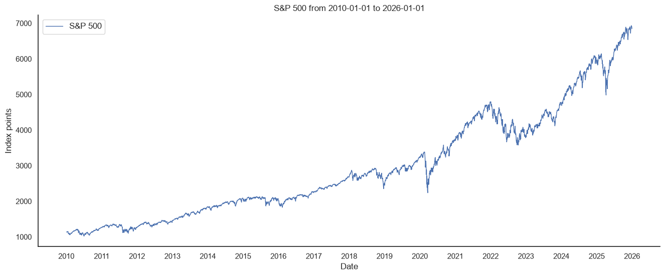

Step #3 Preprocess the Data

Before training the neural network, we split the observations chronologically. The scaler is fitted only on the first 80% so that future price ranges cannot leak into training. Each sample contains 50 daily closes and one target five trading sessions after the final input close.

train_size = int(len(close_prices) * 0.8)

# Fit preprocessing on the training period only to avoid leaking future price ranges.
scaler = MinMaxScaler(feature_range=(0, 1))
scaler.fit(close_prices.iloc[:train_size])
scaled_prices = scaler.transform(close_prices)

sequence_length = 50


def create_direct_horizon_sequences(values, sequence_length, forecast_horizon):
  features, targets, target_indices = [], [], []
  for input_end in range(sequence_length, len(values) - forecast_horizon + 1):
    target_index = input_end + forecast_horizon - 1
    features.append(values[input_end - sequence_length:input_end])
    targets.append(values[target_index, 0])
    target_indices.append(target_index)

  return (
    np.asarray(features, dtype=np.float32),
    np.asarray(targets, dtype=np.float32),
    np.asarray(target_indices),
  )


x_all, y_all, target_indices = create_direct_horizon_sequences(
  scaled_prices,
  sequence_length,
  forecast_horizon,
)
train_mask = target_indices < train_size
x_train, y_train = x_all[train_mask], y_all[train_mask]
x_test, y_test = x_all[~train_mask], y_all[~train_mask]
test_target_indices = target_indices[~train_mask]
test_index = close_prices.index[test_target_indices]

print(f"Training shapes: {x_train.shape}, {y_train.shape}")
print(f"Test shapes: {x_test.shape}, {y_test.shape}")

# The first held-out target is five trading sessions after its final input value.
assert test_target_indices[0] == train_size
assert np.isclose(
  x_test[0, -1, 0],
  scaled_prices[test_target_indices[0] - forecast_horizon, 0],
)
print(
  "First held-out forecast:",
  close_prices.index[test_target_indices[0] - forecast_horizon].date(),
  "->",
  test_index[0].date(),
)

Training shapes: (3165, 50, 1), (3165,)
Test shapes: (805, 50, 1), (805,)
First held-out forecast: 2022-10-10 -> 2022-10-17

Step #4 Building a Time Series Prediction Model

The model receives an input with the shape (50, 1): 50 daily time steps and one feature per step. Two LSTM layers summarize that sequence before the dense layers produce one value for the fixed five-session horizon.

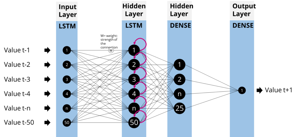
The model architecture of the recurrent neural network

We use the following important arguments for model.fit():

• x_train: Array containing the 50-step input sequences.
• y_train: Array containing the five-session-ahead targets.
• Epochs: The maximum number of times the model passes through the training set.
• Batch size: Integer value that defines the number of samples that will be propagated through the network. After each propagation, the network adjusts the weights of the nodes in each layer.
• Validation split: The final 10% of the training samples are used for chronological validation. We keep shuffle=False so later observations are not mixed into earlier batches.

model = keras.Sequential(
  [
    keras.layers.Input(shape=(sequence_length, 1)),
    keras.layers.LSTM(50, return_sequences=True),
    keras.layers.LSTM(50),
    keras.layers.Dense(25, activation="relu"),
    keras.layers.Dense(1),
  ],
  name="sp500_five_session_lstm",
)
model.compile(optimizer=keras.optimizers.Adam(), loss="mean_squared_error")
model.summary()

early_stopping = keras.callbacks.EarlyStopping(
  monitor="val_loss",
  patience=3,
  restore_best_weights=True,
)
history = model.fit(
  x_train,
  y_train,
  batch_size=32,
  epochs=20,
  validation_split=0.1,
  shuffle=False,
  callbacks=[early_stopping],
  verbose=1,
)

Epoch 1/20 - loss: 0.0011 - val_loss: 0.0034
...
Epoch 7/20 - loss: 0.0016 - val_loss: 0.0031

Step #5 Evaluate Model Performance

Next, we calculate MAE, RMSE, and percentage errors on the held-out period. Metrics need context, especially for a trending price series, so we also compare the LSTM with a persistence baseline. At each forecast origin, persistence simply uses the latest available close as the prediction five sessions later.

y_pred_scaled = model.predict(x_test, verbose=0)
y_pred = scaler.inverse_transform(y_pred_scaled).ravel()
y_test_unscaled = scaler.inverse_transform(y_test.reshape(-1, 1)).ravel()

absolute_percentage_errors = np.abs((y_test_unscaled - y_pred) / y_test_unscaled) * 100
mae = mean_absolute_error(y_test_unscaled, y_pred)
rmse = root_mean_squared_error(y_test_unscaled, y_pred)
mape = absolute_percentage_errors.mean()
median_ape = np.median(absolute_percentage_errors)

# A five-session persistence forecast uses the last close available at each forecast origin.
naive_pred = close_prices["Close"].iloc[
  test_target_indices - forecast_horizon
].to_numpy()
naive_mae = mean_absolute_error(y_test_unscaled, naive_pred)
naive_rmse = root_mean_squared_error(y_test_unscaled, naive_pred)

print(f"LSTM MAE: {mae:.2f} index points")
print(f"LSTM RMSE: {rmse:.2f} index points")
print(f"LSTM MAPE: {mape:.2f}%")
print(f"LSTM median absolute percentage error: {median_ape:.2f}%")
print(f"Persistence baseline MAE: {naive_mae:.2f} index points")
print(f"Persistence baseline RMSE: {naive_rmse:.2f} index points")

evaluation = pd.DataFrame(
  {
    "Actual": y_test_unscaled,
    "LSTM": y_pred,
    "Persistence baseline": naive_pred,
  },
  index=test_index,
)
evaluation["LSTM residual"] = evaluation["LSTM"] - evaluation["Actual"]

_, (ax_price, ax_error) = plt.subplots(
  2,
  1,
  figsize=(16, 9),
  sharex=True,
  gridspec_kw={"height_ratios": [3, 1]},
)
sns.lineplot(data=evaluation[["Actual", "LSTM", "Persistence baseline"]], ax=ax_price)
ax_price.set_title("Five-Session Held-Out Predictions vs. Ground Truth")
ax_price.set_ylabel("S&P 500 index points")

colors = np.where(evaluation["LSTM residual"] >= 0, "#2B8A3E", "#C92A2A")
ax_error.bar(evaluation.index, evaluation["LSTM residual"], width=3, color=colors)
ax_error.axhline(0, color="black", linewidth=1)
ax_error.set_ylabel("LSTM residual")
plt.tight_layout()
plt.show()

LSTM MAE: 436.62 index points
LSTM RMSE: 556.19 index points
LSTM MAPE: 7.52%
LSTM median absolute percentage error: 6.88%
Persistence baseline MAE: 80.45 index points
Persistence baseline RMSE: 107.08 index points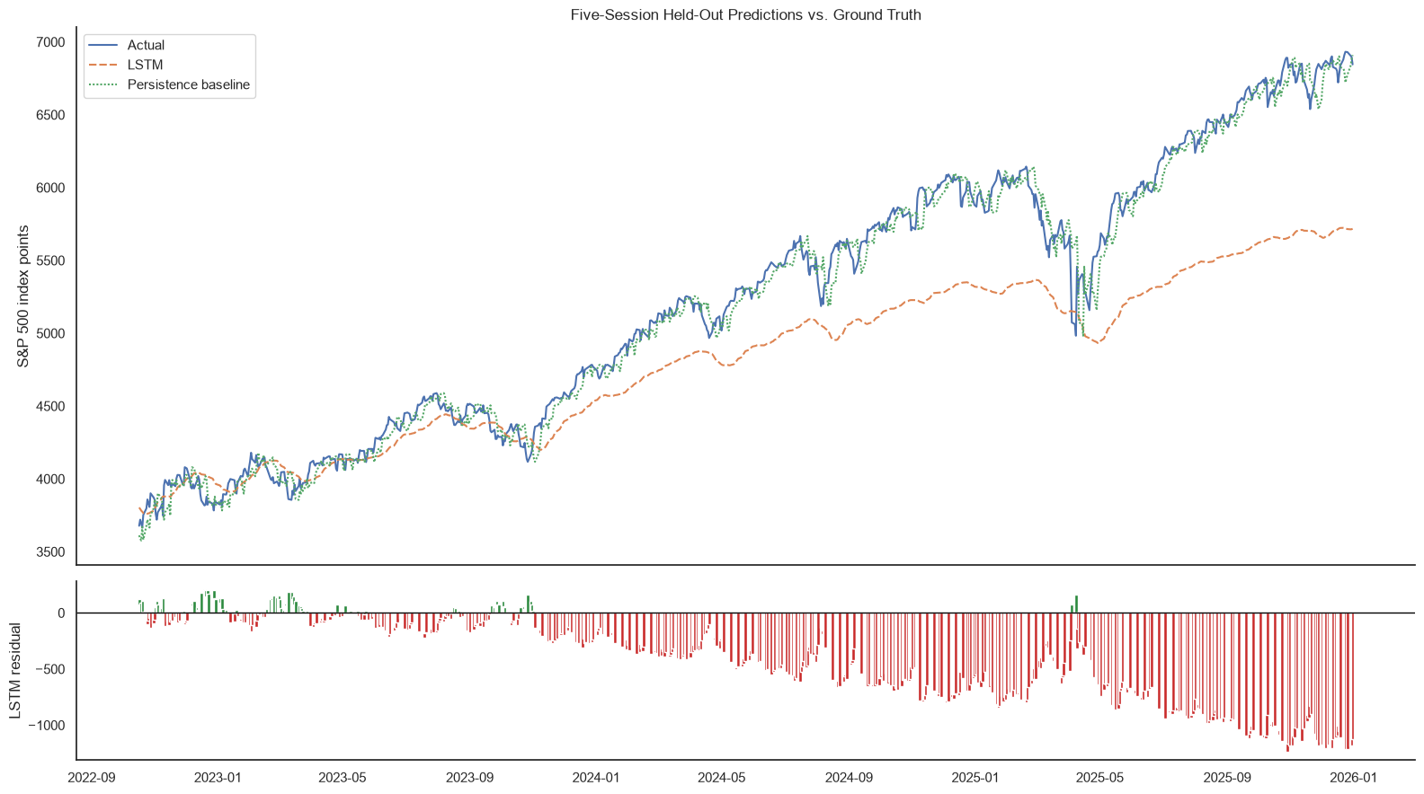

The result is intentionally reported as it is: this LSTM does not beat the simple baseline. Its errors also become increasingly negative as the index rises beyond the price levels represented in training. The direct-horizon alignment is correct, but that alone does not make raw price levels predictable. A serious experiment should consider returns or differences, walk-forward retraining, additional features, and repeated runs across several market regimes.

Step #6 Predict Five Trading Sessions Ahead

Finally, we pass the latest 50 closes to the model. Because the model was trained for one fixed horizon, this output represents the close five trading sessions after the last observation. Given the weak held-out performance, treat it only as an illustration of the API.

last_sequence_scaled = scaler.transform(close_prices.iloc[-sequence_length:])
x_next = last_sequence_scaled[np.newaxis, ...].astype(np.float32)
forecast_close_scaled = model.predict(x_next, verbose=0)
forecast_close = float(scaler.inverse_transform(forecast_close_scaled)[0, 0])

last_date = close_prices.index[-1].date()
last_close = float(close_prices["Close"].iloc[-1])
percent_change = (forecast_close / last_close - 1) * 100

print(f"Last observed {stock_name} close on {last_date}: {last_close:.2f}")
print(
  f"Illustrative {forecast_horizon}-session prediction: "
  f"{forecast_close:.2f} ({percent_change:+.2f}%)"
)

Last observed S&P 500 close on 2025-12-31: 6845.50
Illustrative 5-session prediction: 5736.89 (-16.19%)

The size of this predicted drop is another warning sign, not a trading signal. It is inconsistent with the much stronger persistence baseline and should not be used for financial decisions.

Summary

This article has shown how to change the forecast horizon of a time series model without throwing away daily observations. We shifted each target five trading sessions beyond its input window, fitted preprocessing only on the training period, and evaluated the result against persistence.

The updated experiment also demonstrates why a baseline matters. The LSTM follows the broad direction of the series but performs much worse than simply carrying the latest close forward. Direct, recursive, and multi-output forecasting remain useful strategies, but the horizon design and the model’s predictive value are separate questions.

I hope this article was helpful. Should you have questions or remarks, let me know in the comments.

Sources and Further Readings

The links above to Amazon are affiliate links. By buying through these links, you support the Relataly.com blog and help to cover the hosting costs. Using the links does not affect the price.