Forecasting Beer Sales with ARIMA in Python

Time series analysis and forecasting is a tough nut to crack, but the ARIMA model has been cracking it for decades. ARIMA, short for “autoregressive integrated moving average,” is a powerful statistical modeling technique for time series analysis. It is particularly effective when past values and forecast errors contain useful information about future observations. Seasonal ARIMA extends the model to recurring patterns such as monthly sales cycles. ARIMA has been used to forecast everything from beer sales to order quantities, and this tutorial will show you how to build your own model in Python.

This tutorial proceeds in two parts: The first part covers the concepts behind ARIMA. You will learn how ARIMA works, what Stationarity means, and when it is appropriate to use ARIMA. The second part is a Python hands-on tutorial that applies auto-ARIMA to the Sales Forecasting domain. We’ll be working with a time series of beer sales, and our goal is to predict how the beer sales quantities will evolve in the coming years. First, we check if the time series is stationary. Then we train an ARIMA forecasting model. Finally, we use the model to produce a sales forecast and measure the model’s performance.

About Sales Forecasting

Sales forecasting is a crucial business strategy that involves predicting future sales volumes for a product (for example, beer) or service. It leverages sophisticated statistical and analytical techniques, such as time series analysis or machine learning algorithms, to scrutinize historical sales data. By identifying trends and patterns within this data, businesses can make informed predictions about their future sales performance.

This strategic forecasting plays a pivotal role in business operations. It is instrumental in guiding key decisions surrounding production, inventory management, staffing, and various other operational elements. By honing in on accurate sales forecasting, businesses can strike the perfect balance - maintaining enough inventory to meet customer demand without overproducing or overstocking. This equilibrium ensures a smooth flow in the supply chain and avoids unnecessary costs tied to excess production or storage.

Furthermore, sales forecasting serves as a roadmap for business growth. It aids in identifying potential market opportunities and predicting future sales revenue. This valuable foresight enables businesses to strategically plan their expansion, ensuring resources are optimally utilized and future goals are met. With this in-depth understanding of sales forecasting, businesses can stay ahead of market trends, navigate through business challenges, and ultimately steer towards success.

Businesses rely on sales forecasting to make informed decisions about production, inventory management, staffing, and other key operational aspects. Image created with Midjourney

Introduction to ARIMA Time Series Modelling

ARIMA models provide an alternative approach to time series forecasting that differs significantly from machine learning methods. Working with ARIMA requires a good understanding of Stationarity and knowledge of the transformations used to make time-series data stationary. The concept of Stationarity is, therefore, first on our schedule.

The Concept of Stationarity

Stationarity is an essential concept in stochastic processes that describes the nature of a time series. We consider a time series strictly stationary if its statistical properties do not change over time. In this case, summary statistics, such as the mean and variance, do not change over time. However, the time-series data we encounter in the real world often show a trend or significant irregular fluctuations, making them non-stationary or weakly stationary.

So why is Stationarity such an essential concept for ARIMA? The model assumes that, after any required differencing, the relationships it estimates remain stable over time. A non-stationary series is not necessarily random or unpredictable. It can contain a trend, changing variance, seasonality, or a unit root. These properties must be modeled or transformed before the AR and MA terms can be interpreted reliably.

Fortunately, in many cases, it is possible to transform a time series that is non-stationary into a stationary form and, in this way, build better prediction models.

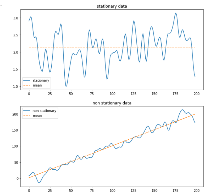
A stationary Vs. a non-stationary time series

How to Test Whether a Time Series is Stationary

The first step in the ARIMA modeling approach is determining whether a time series is stationary. There are different ways to determine whether a time series is stationary:

• Plotting: We can plot the time series and visually check if it shows consistent behavior or changes over a more extended period.
• Summary statistics: We can split the time series into different periods and calculate the summary statistics, such as the variance. If these metrics are subject to significant changes, the time series is non-stationary. However, the results will also depend on the respective periods, leading to false conclusions.
• Statistical tests: Tests such as Kwiatkowski-Phillips-Schmidt-Shin, Augmented Dickey-Fuller, and Phillips-Perron evaluate specific forms of non-stationarity. Their null hypotheses differ, so the result must be interpreted in the context of the chosen test. In the ADF test used below, the null hypothesis is that the series has a unit root.

What is an (S)ARIMA Model?

As the name implies, ARIMA uses autoregression (AR), integration (differencing), and moving averages (MA) to fit a linear regression model to a time series.

ARIMA Parameters

The default notation for ARIMA is a model with parameters p, d, and q, whereby each parameter takes an integer value:

• d (differencing): In the case of a non-stationary time series, there is a chance to remove a trend from the data by differencing once or several times, thus bringing the data to a stationary state. The model parameter d determines the order of the differentiation. A value of d = 0 simplifies the ARIMA model to an ARMA model, lacking the integration aspect. If this is the case, we do not need to integrate the function because the time series is already stationary.
• p (order of the AR terms): The autoregressive process describes the dependent relationship between an observation and several lagged observations (lags). Predictions are then based on past data from the same time series using linear functions. p = 1 means the model uses values that lag by one period.
• q (order of the MA terms): The parameter q determines the number of lagged forecast errors in the prediction equation. In contrast to the AR process, the MA process assumes that values at a future point in time depend on the errors made by predictions at current and past points in time. This means that it is not previous events that determine the predictions but rather the previous estimation or prediction errors used to calculate the following time series value.

SARIMA

In the real world, many time series have seasonal effects. Examples are monthly retail sales figures, temperature reports, weekly airline passenger data, etc. To consider this, we can specify a seasonal range (e.g., m=12 for monthly data) and additional seasonal AR or MA components for our model that deal with seasonality. Such a model is also called a SARIMA model, and we can define it as a model(p, d, q)(P, D, Q)[m].

Auto-(S)ARIMA

When working with ARIMA, we can set the model parameters manually or use auto-ARIMA to search a defined parameter space. With the seasonal option enabled, the process also evaluates seasonal components. Auto-ARIMA uses differencing tests to help determine the order of ordinary differencing, d, then fits candidate models within ranges such as start_p to max_p and start_q to max_q. Seasonal tests and parameter ranges perform the same role for D, P, and Q. The final model is selected using an information criterion such as AIC, so its residuals and held-out forecast performance still need to be checked.

Creating a Sales Forecast with ARIMA in Python

Having grasped the fundamental concepts behind ARIMA (AutoRegressive Integrated Moving Average), we’re now ready to dive into the practical aspect of crafting a sales forecasting model in Python. Utilizing ARIMA for forecasting sales data is an esteemed practice owing to the algorithm’s adeptness in modeling seasonal changes combined with long-term trends - a characteristic commonly exhibited by sales data.

In this tutorial, we’ll be employing a dataset representing the monthly beer sales across the United States from 1992 through 2018, recorded in millions of US dollars. Our objective is to construct a robust time series model using ARIMA to accurately predict future sales trends.

When it comes to the technological aspect, we’ll be using the Python-based ‘statsmodels’ and ‘pmdarima’ libraries to build our ARIMA sales forecasting model. So, if you’re ready to harness the power of Python and ARIMA for sales prediction, let’s get started!

The code is available on the GitHub repository.

A fluffy cat drinking beer after creating an ARIMA sales forecast. Image created with Midjourney

Prerequisites

Before we start coding, ensure you have set up your Python 3 environment and required packages. If you don’t have an environment, you can follow this tutorial to set up the Anaconda environment.

Also, make sure you install all required packages. The refreshed tutorial was tested with Python 3.12, pandas 3.0, statsmodels 0.14, pmdarima 2.1, NumPy 2.5, matplotlib 3.11, and seaborn 0.13. It uses the following standard packages:

• pandas
• NumPy
• matplotlib

In addition, we will be using the statsmodels library and pmdarima.

You can install packages using console commands:

• pip install
• conda install  (if you are using the anaconda packet manager)

Step #1 Load the Sales Data to Our Python Project

In the initial step, we set up the Python environment and load monthly beer sales in the United States from 1992 through 2018. The original remote CSV is no longer available, so the GitHub tutorial now contains a repository-local copy of the dataset cited from Kaggle. The path lookup works when the notebook kernel starts in either the repository root or the notebook’s subfolder.

# A tutorial for this file is available at www.relataly.com
# Tested with Python 3.12, pandas 3.0, statsmodels 0.14, and pmdarima 2.1

from pathlib import Path

import matplotlib.pyplot as plt
import pandas as pd
import pmdarima as pm
import seaborn as sns
from statsmodels.graphics.tsaplots import plot_acf
from statsmodels.tsa.seasonal import seasonal_decompose

sns.set_theme(style="white", rc={"axes.spines.right": False, "axes.spines.top": False})

# Originally published at:
# https://www.kaggle.com/datasets/bulentsiyah/for-simple-exercises-time-series-forecasting
relative_data_path = Path("data/alcohol_sales/BeerWineLiquor.csv")
data_path = next(
  path / relative_data_path
  for path in (Path.cwd(), *Path.cwd().parents)
  if (path / relative_data_path).exists()
)
df = pd.read_csv(data_path, parse_dates=["date"], date_format="%m/%d/%Y")
df.head()

		date	beer
0	1/1/1992	1509
1	2/1/1992	1541
2	3/1/1992	1597
3	4/1/1992	1675
4	5/1/1992	1822

As shown above, the sales figures in this dataset stem from the first day of each month.

Step #2 Visualize the Time Series and Check it for Stationarity

Before modeling the sales data, we visualize the time series and test it for Stationarity. Visualization helps us choose the parameters for our ARIMA model, thus making it an essential step.

First, we will look at the different components of the time series. We do this by using the seasonal_decompose function of the statsmodels library.

# Decompose the time series
plt.rcParams["figure.figsize"] = (10,6)
result = seasonal_decompose(df['beer'], model='multiplicative', period = 12)
result.plot()
plt.show()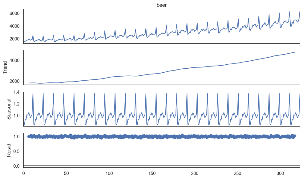

To test for Stationarity, we use the ADFuller test. It is common to run this test multiple times throughout a data science project. Therefore, we create a function that we can then reuse later.

def check_stationarity(sales, title_string):
    sales = sales.dropna().rename("beer")
    plot_data = sales.to_frame()

    if sales.size > 12:
        plot_data["12-month moving average"] = sales.rolling(window=12).mean()
        plot_data["25-month moving average"] = sales.rolling(window=25).mean()

    _, ax = plt.subplots(figsize=(16, 8))
    sns.lineplot(data=plot_data, ax=ax, palette=sns.color_palette("mako_r", plot_data.shape[1]))
    ax.set_title(title_string, fontsize=14)
    ax.legend(title="Series", loc="upper left")
    plt.show()

    # ADFTest returns the p-value and whether differencing is recommended at alpha=0.05.
    adf_test = pm.arima.ADFTest(alpha=0.05)
    p_value, should_difference = adf_test.should_diff(sales)
    print(f"ADF p-value: {p_value:.4f}; should difference: {should_difference}")


df_sales = df.set_index("date")[["beer"]].sort_index().asfreq("MS")
title = "Beer sales in the US between 1992 and 2018 in million US$/month"
check_stationarity(df_sales["beer"], title)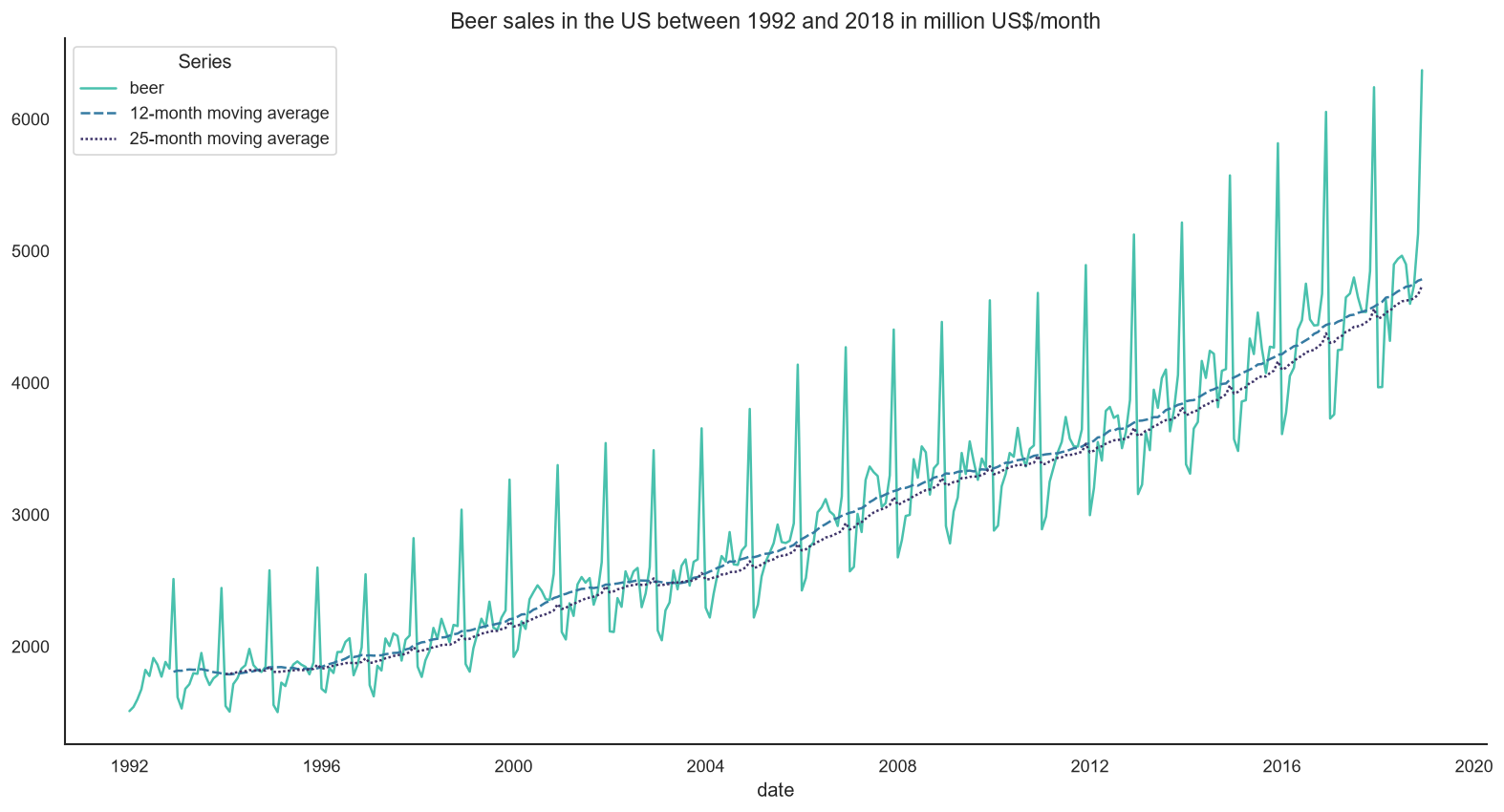

The chart shows a rising level and strong annual seasonality. However, the ADF test returns a p-value of 0.0191 and should difference: False, so it rejects its unit-root null hypothesis at the 5% level and does not recommend ordinary differencing. This result does not mean the seasonal structure can be ignored. The model search below selects d=0 for ordinary differencing and D=1 for seasonal differencing. Also note that these figures represent sales value, so the increase should not be interpreted directly as growth in physical beer consumption.

Step #3 Exemplary Differencing and Autocorrelation

The chart from the previous section shows a changing level and a pronounced seasonal component. The ADF test does not find evidence for an ordinary unit root, but the yearly pattern still needs to be represented. We therefore search both ordinary and seasonal SARIMA parameters.

Before we use auto-correlation to determine the optimal parameters, we will try manual differencing to make the time series stationary. There is no guarantee that differencing works. It is essential to remember that differencing can sometimes also worsen prediction performance. So be careful, not to overdifference! We could also trust that the auto-ARIMA model chooses the best parameters for us. However, we should always validate the selected parameters.

The ideal differencing parameter is the least number of differencing steps to achieve a stationary time series. We will monitor the results with autocorrelation plots to check whether differencing was successful.

We print the autocorrelation for the original time series and after the first and second-order differencing.

# 3.1 Non-seasonal part
def auto_correlation(df, prefix, lags):
    plt.rcParams.update({'figure.figsize':(7,7), 'figure.dpi':120})

    # Define the plot grid
    _, axes = plt.subplots(3,2, sharex=False)

    # Original series
    axes[0, 0].plot(df)
    axes[0, 0].set_title('Original' + prefix)
    plot_acf(df, lags=lags, ax=axes[0, 1])

    # First Difference
    df_first_diff = df.diff().dropna()
    axes[1, 0].plot(df_first_diff)
    axes[1, 0].set_title('First Order Difference' + prefix)
    plot_acf(df_first_diff, lags=lags - 1, ax=axes[1, 1])

    # Second Difference
    df_second_diff = df.diff().diff().dropna()
    axes[2, 0].plot(df_second_diff)
    axes[2, 0].set_title('Second Order Difference' + prefix)
    plot_acf(df_second_diff, lags=lags - 2, ax=axes[2, 1])
    plt.tight_layout()
    plt.show()

auto_correlation(df_sales['beer'], '', 10)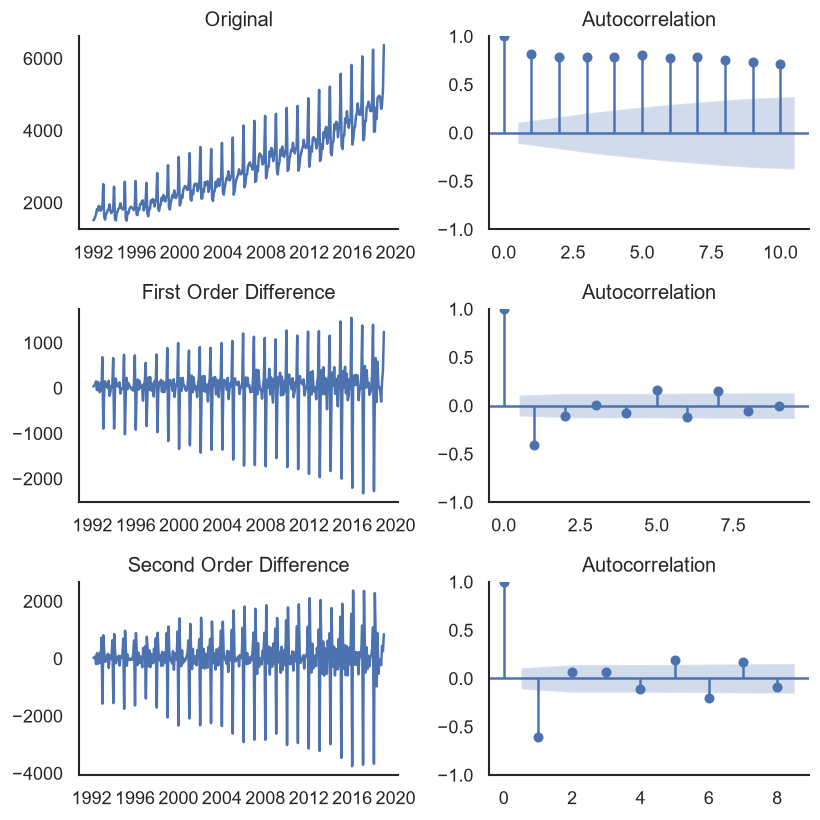

The ACF after first-order differencing turns negative immediately at lag one. That pattern is a warning that ordinary differencing may remove too much structure. This agrees with the earlier ADF result and gives us a reason to allow d=0 in the model search.

Next, we calculate a true seasonal difference. For monthly data, this means subtracting the value from the same month one year earlier across the full time series. Taking ordinary differences within a single year would not estimate the seasonal differencing parameter D.

# 3.2 Seasonal differencing
seasonal_lag = 12
seasonal_difference = df_sales["beer"].diff(seasonal_lag).dropna()

fig, axes = plt.subplots(1, 2, figsize=(12, 4))
axes[0].plot(seasonal_difference)
axes[0].set_title("Difference from the same month one year earlier")
plot_acf(seasonal_difference, lags=24, ax=axes[1])
plt.tight_layout()
plt.show()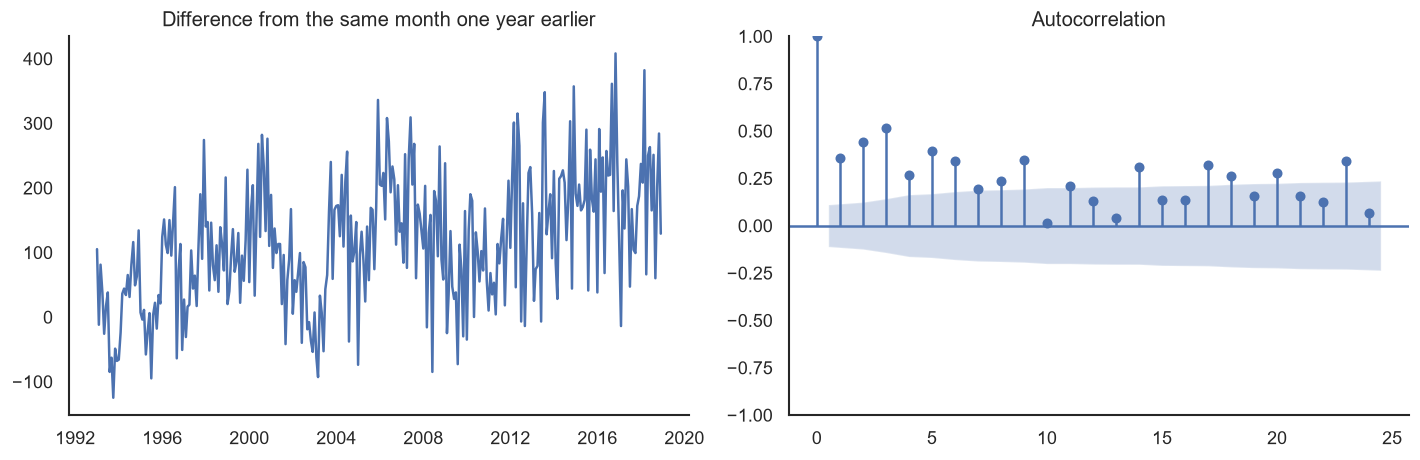

# Test the lag-12 seasonal difference for a remaining unit root.
check_stationarity(seasonal_difference, "Seasonally Differenced Beer Sales")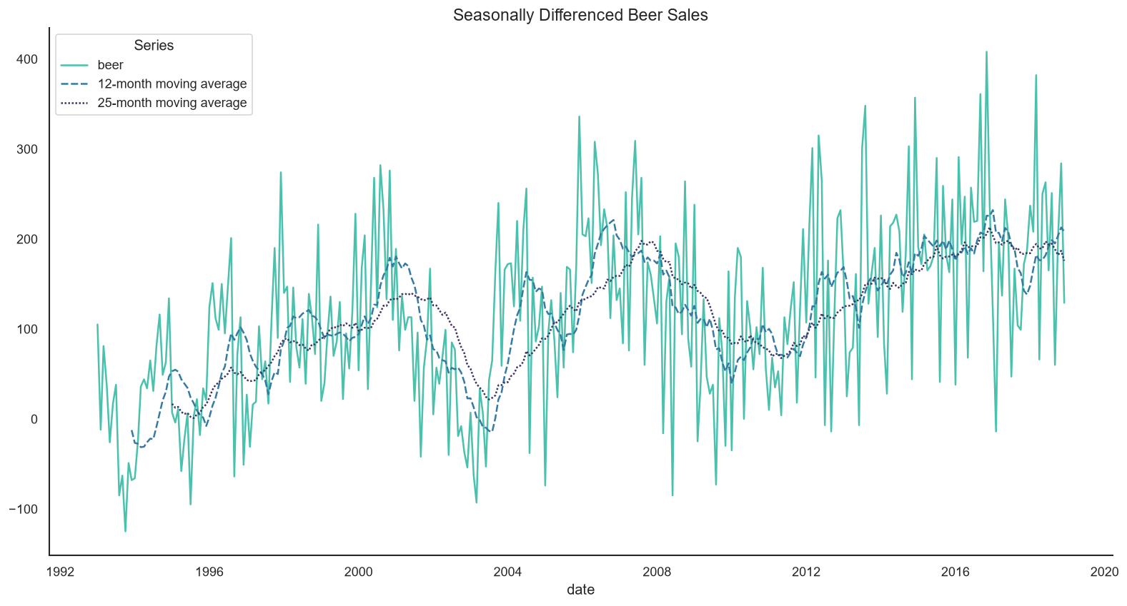

ADF p-value: 0.0100; should difference: False

After lag-12 seasonal differencing, the ADF test rejects its unit-root null hypothesis and recommends no additional ordinary differencing. This supports searching a model with one seasonal difference (D=1) while keeping ordinary differencing optional.

Step #4 Finding an Optimal Model with Auto-ARIMA

Next, we auto-fit an ARIMA model to our time series. In this way, we ensure that we can later measure the performance of our model against a fresh set of data that the model has not seen so far. We will split our dataset into train and test in preparation for this.

Once we have created the train and test datasets, we configure the auto_arima stepwise optimization. The search considers ordinary AR, differencing, and MA orders up to three. The ADF test helps choose ordinary differencing within that range.

To deal with the seasonality, we set seasonal=True and m=12. This turns the search into a SARIMA search with additional D, P, and Q parameters. We let the optimizer test seasonal AR and MA orders up to three and seasonal differencing up to two. The selected model should then be judged on its diagnostics and on the untouched final 30 months.

After configuring the parameters, we next fit the model to the time series. The model will try to find the optimal parameters and choose the model with the least AIC.

# Reserve the final 30 months as an untouched test set.
pred_periods = 30
split_number = len(df_sales) - pred_periods
df_train = df_sales.iloc[:split_number].rename(columns={"beer": "y_train"}).copy()
df_test = df_sales.iloc[split_number:].rename(columns={"beer": "y_test"}).copy()

model_fit = pm.auto_arima(
  df_train["y_train"],
  test="adf",
  max_p=3,
  max_d=3,
  max_q=3,
  seasonal=True,
  m=12,
  max_P=3,
  max_D=2,
  max_Q=3,
  trace=True,
  error_action="ignore",
  suppress_warnings=True,
  stepwise=True,
)

print(model_fit.summary())

Performing stepwise search to minimize aic
 ARIMA(2,0,2)(1,1,1)[12] intercept   : AIC=inf, Time=3.89 sec
 ARIMA(0,0,0)(0,1,0)[12] intercept   : AIC=3383.210, Time=0.02 sec
 ARIMA(1,0,0)(1,1,0)[12] intercept   : AIC=3351.655, Time=0.38 sec
 ARIMA(0,0,1)(0,1,1)[12] intercept   : AIC=3364.350, Time=1.09 sec
 ARIMA(0,0,0)(0,1,0)[12]             : AIC=3604.145, Time=0.02 sec
 ARIMA(1,0,0)(0,1,0)[12] intercept   : AIC=3349.908, Time=0.11 sec
 ARIMA(1,0,0)(0,1,1)[12] intercept   : AIC=3351.532, Time=0.29 sec
 ARIMA(1,0,0)(1,1,1)[12] intercept   : AIC=3353.520, Time=1.24 sec
 ARIMA(2,0,0)(0,1,0)[12] intercept   : AIC=3312.656, Time=0.10 sec
 ARIMA(2,0,0)(1,1,0)[12] intercept   : AIC=3314.483, Time=0.57 sec
 ARIMA(2,0,0)(0,1,1)[12] intercept   : AIC=3314.378, Time=0.30 sec
 ARIMA(2,0,0)(1,1,1)[12] intercept   : AIC=3305.552, Time=3.02 sec
 ARIMA(2,0,0)(2,1,1)[12] intercept   : AIC=3291.425, Time=4.19 sec
 ARIMA(2,0,0)(2,1,0)[12] intercept   : AIC=3306.914, Time=3.06 sec
 ARIMA(2,0,0)(3,1,1)[12] intercept   : AIC=3276.501, Time=4.67 sec
 ARIMA(2,0,0)(3,1,0)[12] intercept   : AIC=3282.240, Time=5.24 sec
 ARIMA(2,0,0)(3,1,2)[12] intercept   : AIC=inf, Time=7.39 sec
 ARIMA(2,0,0)(2,1,2)[12] intercept   : AIC=inf, Time=4.74 sec
 ARIMA(1,0,0)(3,1,1)[12] intercept   : AIC=3313.877, Time=5.17 sec
 ARIMA(3,0,0)(3,1,1)[12] intercept   : AIC=3246.820, Time=5.72 sec
 ARIMA(3,0,0)(2,1,1)[12] intercept   : AIC=3255.313, Time=5.33 sec
 ARIMA(3,0,0)(3,1,0)[12] intercept   : AIC=3249.998, Time=6.77 sec
 ARIMA(3,0,0)(3,1,2)[12] intercept   : AIC=inf, Time=8.39 sec
 ARIMA(3,0,0)(2,1,0)[12] intercept   : AIC=3259.938, Time=3.55 sec
...
===================================================================================

Warnings:
[1] Covariance matrix calculated using the outer product of gradients (complex-step).

With pmdarima 2.1, auto-ARIMA selects SARIMA(3,0,0)(3,1,1)[12] with an intercept and an AIC of 3246.82. Its d=0, D=1 differencing orders agree with the diagnostics in section 3.

Step #5 Simulate the Time Series using in-sample Forecasting

Now that we have trained our model, we use predict_in_sample to calculate one-step-ahead fitted values for the training period. These values are useful for diagnostics, but they are not a substitute for the held-out forecast in the next section. We omit the first seasonal cycle from the chart because model initialization dominates those early fitted values.

# Generate one-step-ahead in-sample predictions.
in_sample_prediction = model_fit.predict_in_sample(dynamic=False)
df_train["y_train_pred"] = in_sample_prediction

df_train["absolute_percentage_error"] = (
  (df_train["y_train"] - df_train["y_train_pred"]).abs() / df_train["y_train"] * 100
)

# Skip the first seasonal cycle, where model initialization dominates the fitted values.
plot_data = df_train.iloc[12:]
fig, ax1 = plt.subplots(figsize=(16, 8))
sns.lineplot(data=plot_data[["y_train", "y_train_pred"]], ax=ax1, linewidth=1.0)
ax1.set_title("In-Sample Sales Prediction", fontsize=14)

ax2 = ax1.twinx()
ax2.set_ylabel("Absolute percentage error", color="purple", fontsize=14)
ax2.set_ylim(0, 50)
ax2.bar(
  plot_data.index,
  plot_data["absolute_percentage_error"],
  width=20,
  color="purple",
  alpha=0.35,
  label="Absolute percentage error",
)
ax2.legend(loc="upper right")
plt.show()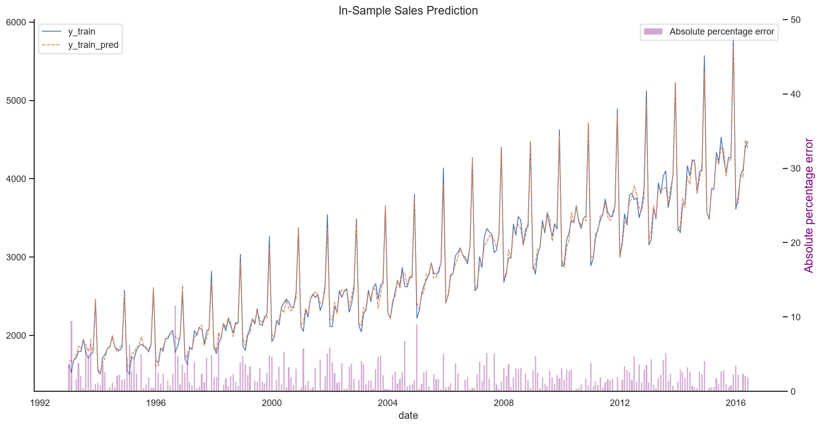

Next, we take a look at the prediction errors.

Step #6 Generate and Visualize a Sales Forecast

Now we forecast the 30 months that were excluded from training. Because df_test already has the correct monthly index, pandas aligns the returned predictions directly with the observed values. The vertical line makes the train/test boundary explicit.

# Forecast the held-out 30 months after the end of the training data.
df_test["y_test_pred"] = model_fit.predict(n_periods=pred_periods)
df_union = pd.concat([df_train, df_test])

fig, ax = plt.subplots(figsize=(16, 8))
sns.lineplot(
  data=df_union[["y_train", "y_train_pred", "y_test", "y_test_pred"]],
  ax=ax,
  linewidth=1.0,
  dashes=False,
  palette="muted",
)
ax.axvline(df_test.index[0], color="black", linestyle="--", linewidth=1, label="Test period starts")
ax.set_title("Training Fit and Held-Out Forecast", fontsize=14)
ax.set_xlim(df_union.index[150], df_union.index.max())
ax.legend()
sns.despine()
plt.show()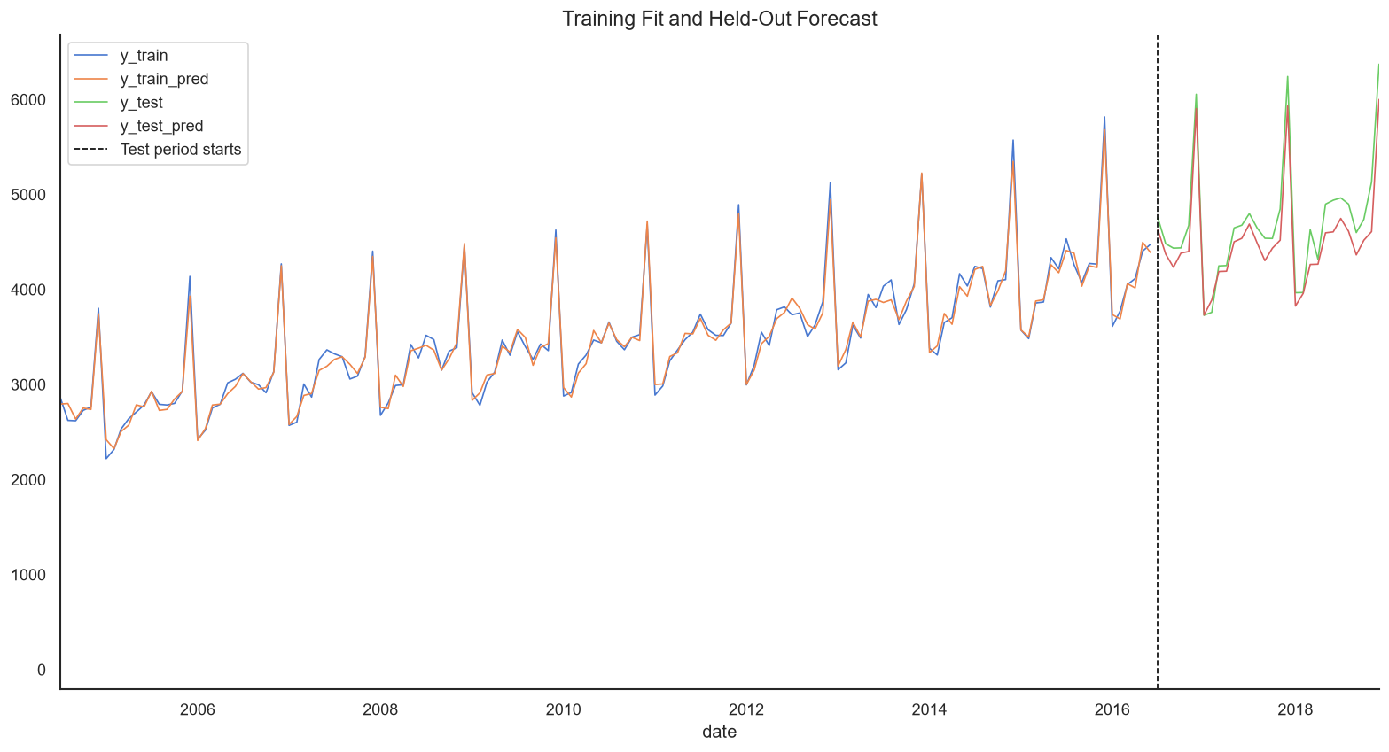

As shown above, the forecast continues the historical seasonal pattern and follows the held-out observations reasonably closely. This is evidence about performance from July 2016 through December 2018. It should not be treated as a forecast of current beer sales because the dataset ends in 2018.

Step #7 Measure the Performance of the Sales Forecasting Model

In this section, we will measure the performance of our ARIMA model. To learn more about this topic, check out this relataly article measuring regression performance.

The previous chart shows a few larger prediction errors. Two useful summaries are the mean absolute percentage error (MAPE) and the median absolute percentage error. The median is less sensitive to unusually large misses.

absolute_percentage_errors = (
  (df_test["y_test"] - df_test["y_test_pred"]).abs() / df_test["y_test"] * 100
)
mape = absolute_percentage_errors.mean()
median_ape = absolute_percentage_errors.median()

print(f"Mean Absolute Percentage Error (MAPE): {mape:.2f}%")
print(f"Median Absolute Percentage Error: {median_ape:.2f}%")

Mean Absolute Percentage Error (MAPE): 3.94%
Median Absolute Percentage Error: 3.49%

Across the held-out 30 months, the average absolute error is 3.94% and the median is 3.49%. These values are specific to this historical split; a production forecast should also use rolling-origin evaluation and prediction intervals.

Summary

This Python tutorial has shown how to use SARIMA for sales forecasting. Sales forecasts can inform production, inventory management, staffing, and growth planning. Here, we used historical US beer sales value to demonstrate seasonal diagnostics, model selection, in-sample checks, and a held-out evaluation.

In the first part, we learned how ARIMA works, what stationarity means, and how an ADF test and autocorrelation plots inform differencing choices. In the second part, auto-ARIMA selected SARIMA(3,0,0)(3,1,1)[12]. The resulting forecast achieved a MAPE of 3.94% on the final 30 months of this dataset.

If you have any questions or suggestions, please let me know in the comments, and I will do my best to answer.

Now that you have learned to use ARIMA to forecast beer sales, you really earned yourself a beer. Cheers! Image created with Midjourney

Sources and Further Reading

1. Charu C. Aggarwal (2018) Neural Networks and Deep Learning
2. Jansen (2020) Machine Learning for Algorithmic Trading: Predictive models to extract signals from market and alternative data for systematic trading strategies with Python
3. Aurélien Géron (2019) Hands-On Machine Learning with Scikit-Learn, Keras, and TensorFlow: Concepts, Tools, and Techniques to Build Intelligent Systems
4. David Forsyth (2019) Applied Machine Learning Springer
5. Andriy Burkov (2020) Machine Learning Engineering

The links above to Amazon are affiliate links. By buying through these links, you support the Relataly.com blog and help to cover the hosting costs. Using the links does not affect the price.

Want to learn more about time series analysis and prediction? Check out these recent relataly tutorials:

• Stock Market Prediction - Building a Univariate Model using Keras Recurrent Neural Networks in Python.
• Building Multivariate Time Series Models for Stock Market Prediction with Python
• Time Series Forecasting - Creating a Multi-Step Forecast in Python
• Python Cheat Sheet: Measuring Prediction Errors in Time Series Forecasting
• Evaluate Time Series Forecasting Models with Python