Univariate Stock Market Forecasting using Facebook Prophet in Python

Have you ever wondered how a forecasting model can combine a changing trend with recurring seasonal patterns? Meet Prophet, the open-source time series forecasting library originally developed by Facebook’s Core Data Science team. The current Python package is called prophet and uses CmdStanPy for model fitting. Prophet offers a compact interface and a modular model with trend, seasonality, holiday, and optional regressor components. It is particularly useful as an interpretable baseline for time series with several seasons of history.

We begin with a brief discussion of how Prophet decomposes a time series into different components. Then we turn to the hands-on part and generate a forecast from Coca-Cola’s adjusted closing price. More importantly, we reserve recent observations for a chronological backtest and compare Prophet with a simple last-value baseline before fitting the final forecast.

Disclaimer: This article does not constitute financial advice. Stock markets can be very volatile and are generally difficult to predict. Predictive models and other forms of analytics applied in this article only illustrate machine learning use cases.

Facebook Prophet - an open-source tool for time series forecasting

What is Facebook Prophet?

Prophet is a forecasting library introduced by Taylor and Letham, 2017 and later released as an open-source project. It was designed for business time series that contain trend changes, seasonal patterns, and known events. Its defaults make a first model easy to fit, but they do not remove the need for domain knowledge, chronological validation, suitable baselines, and parameter tuning. Before we dive into the hands-on part, let’s gain a quick overview of how Prophet works.

Also: Stock Market Prediction using Multivariate Time Series

Time-series forecasting with Facebook Prophet. Image generated with Midjourney.

How Facebook Prophet Works

Prophet uses an additive regression model that combines several components:

• Trends
• Seasonality
• Holidays and other known events

The trend describes long-term growth or decline, while Fourier-series terms model recurring seasonal patterns. Holiday and regressor effects can be supplied when they are known for both training and future dates. Prophet combines these terms with an error component to form the forecast. Unlike an autoregressive model, standard Prophet does not directly use lagged target values or automatically assign decreasing weights to older observations.

A) Dealing with Trends

Time series often have a trendline, but a single slope may not describe the complete history. Prophet distributes potential changepoints across a configurable part of the training period and regularizes the slope adjustments at those points. Its built-in growth options are linear, logistic, and flat. You can also supply changepoint dates manually when domain knowledge supports them.

B) Seasonality

Prophet can model strong seasonal patterns with Fourier-series terms made from sine and cosine functions. Its automatic settings enable seasonalities only when the history supports them; for example, yearly seasonality needs at least two years of data. Custom seasonalities can be added for patterns that the defaults do not represent.

C) Holiday

Public holidays and promotions can lead to repeatable deviations in demand or traffic. Prophet lets us supply these dates so the model can estimate their effects. The same mechanism can represent other known events. Prophet tolerates missing timestamps, but it does not automatically identify and remove outliers; unusual observations should be investigated and corrected or marked when appropriate.

Hyperparameter Tuning and Customization

Prophet provides regularized defaults rather than automatic Bayesian hyperparameter optimization. Parameters such as changepoint_prior_scale, seasonality_prior_scale, and changepoint_range should be evaluated with rolling or chronological validation. Prophet also includes cross-validation, diagnostics, and visualization helpers.

Also: Using Random Search to Tune the Hyperparameters of a Random Decision Forest with Python

Application Domains

Prophet is applicable in several domains, especially when trend, seasonality, and known calendar events explain a meaningful share of the variation. Possible applications include:

• Sales forecasting: Facebook Prophet can be used to predict future sales of a product or service, based on historical sales data. This can be useful for businesses to plan their inventory and staffing, and to make informed decisions about future investments and growth.
• Financial forecasting: Prophet can provide an interpretable benchmark for prices or volumes, although financial markets are noisy and a seasonal trend model should not be assumed to create an investment edge.
• Traffic forecasting: Facebook Prophet can be used to predict future traffic on a website or mobile app based on historical data. This can be useful for businesses to plan for capacity and optimize their servers and infrastructure.
• Energy consumption forecasting: Facebook Prophet can be used to predict future energy consumption based on historical data. This can be useful for utilities and energy companies to plan for demand and optimize their generation and distribution.

When to Use Facebook Prophet?

Prophet is most effective when a time series has a stable frequency, several seasons of history, interpretable trend changes, and known events that may influence the target. It is less suitable when short-term autoregressive effects dominate, when the data-generating process changes abruptly, or when only a small amount of history is available. Always compare it with simple baselines on unseen dates.

Also: Rolling Time Series Forecasting: Creating a Multi-Step Prediction

Using Facebook Prophet to Forecast the Coca-Cola Stock Price in Python

In this hands-on tutorial, we’ll use Prophet and Python to create a forecast for Coca-Cola’s adjusted closing price. Coca-Cola is generally considered a defensive consumer-staples stock, not a cyclical stock. We use it because the long history contains trend changes and because its limited predictability makes validation especially important. This involves the following steps:

1. Collect historical stock data for CocaCola and familiarize ourselves with the data.
2. Reserve the most recent 126 observations as a chronological holdout.
3. Fit Prophet and compare its holdout errors with a constant last-value forecast.
4. Refit the model on all observations and generate a future forecast.
5. Visualize the model components and compare changepoint windows.

The result is an educational model comparison, not a claim about the future performance of Coca-Cola stock. Let’s get started!

As always, you can find the code of this tutorial on the GitHub repository.

Prerequisites

Before you proceed, ensure that you have set up a recent Python environment and the required packages. This tutorial was refreshed with Python 3.12, Prophet 1.3, pandas 3.0, scikit-learn 1.9, and yfinance 1.5. If you don’t have an environment, consider following this tutorial to set up an Anaconda environment.

Install the required packages with pip. Current Prophet wheels include the compiled model support needed for normal use, so this tutorial does not call cmdstanpy.install_cmdstan() at runtime.

pip install matplotlib numpy pandas prophet scikit-learn yfinance

Step #1 Loading Packages and Data

Let’s begin by loading the required Python packages and historical Coca-Cola prices from Yahoo Finance. We use a fixed date range instead of today’s date so later runs cover the same period. The end argument is exclusive, which is why 2026-01-01 includes observations through 2025-12-31. We also set auto_adjust=True, so the Close column is adjusted for splits and dividends. Yahoo Finance can still revise historical values after corporate actions.

import logging
import warnings
from importlib.metadata import version

warnings.filterwarnings("ignore", message="IProgress not found.*")

import matplotlib.pyplot as plt
import numpy as np
import pandas as pd
import yfinance as yf
from prophet import Prophet
from prophet.plot import add_changepoints_to_plot
from sklearn.metrics import mean_absolute_error, root_mean_squared_error

cmdstan_logger = logging.getLogger("cmdstanpy")
if not cmdstan_logger.handlers:
  cmdstan_logger.addHandler(logging.NullHandler())
cmdstan_logger.setLevel(logging.WARNING)
plt.style.use("seaborn-v0_8-whitegrid")

SYMBOL = "KO"
STOCK_NAME = "Coca-Cola"
START_DATE = "2015-01-01"
END_DATE = "2026-01-01"  # yfinance treats end as exclusive

prices = yf.download(
  SYMBOL,
  start=START_DATE,
  end=END_DATE,
  auto_adjust=True,
  multi_level_index=False,
  progress=False,
)
if prices.empty:
  raise RuntimeError("Yahoo Finance returned no data. Check the connection and ticker.")

print(f"pandas {pd.__version__}, Prophet {version('prophet')}, yfinance {yf.__version__}")
prices.head()

pandas 3.0.3, Prophet 1.3.0, yfinance 1.5.1

Once we have downloaded the data, we create a line plot of the adjusted closing price. Prophet needs one target column, although it can also include holidays and additional regressors. For illustration purposes, we add a moving average to the chart. It makes longer movements easier to spot but will not be used to fit the model.

rolling_window = 25
moving_average = prices["Close"].rolling(rolling_window).mean()

fig, ax = plt.subplots(figsize=(12, 4))
ax.plot(prices.index, prices["Close"], color="skyblue", linewidth=0.8, label="Adjusted close")
ax.plot(prices.index, moving_average, color="royalblue", linestyle="--", label=f"{rolling_window}-day average")
ax.set(title=f"{STOCK_NAME} adjusted closing price", ylabel="USD", xlabel=None)
ax.legend(frameon=False)
fig.tight_layout()
plt.show()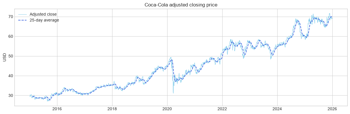

The chart shows a long-term upward trend interrupted by downturns and changes in slope. Visual patterns alone do not establish that future returns are predictable, so we will test the fitted model on unseen dates.

Step #2 Preparing the Data

Next, we prepare the data and create a chronological holdout. Prophet requires the following column names; their order and the dataframe index do not matter:

• ds for the timestamp
• y for the numeric target, which in our case is the adjusted closing price

We reserve the most recent 126 observed market sessions for evaluation. The model will not see these values during training.

HOLDOUT_SIZE = 126

prophet_data = (
  prices[["Close"]]
  .rename(columns={"Close": "y"})
  .rename_axis("ds")
  .reset_index()
  .dropna()
)
prophet_data["ds"] = pd.to_datetime(prophet_data["ds"]).dt.tz_localize(None)
prophet_data = prophet_data.sort_values("ds").drop_duplicates("ds").reset_index(drop=True)

if len(prophet_data) <= HOLDOUT_SIZE:
  raise ValueError("Not enough observations for the requested holdout.")

train_data = prophet_data.iloc[:-HOLDOUT_SIZE].copy()
test_data = prophet_data.iloc[-HOLDOUT_SIZE:].copy()
assert train_data["ds"].max() < test_data["ds"].min()

pd.DataFrame(
  {
    "rows": [len(prophet_data)],
    "train_end": [train_data["ds"].max().date()],
    "holdout_start": [test_data["ds"].min().date()],
    "holdout_end": [test_data["ds"].max().date()],
  }
)

   rows   train_end holdout_start holdout_end
0  2766  2025-07-02    2025-07-03  2025-12-31

Now we have a simple ds/y dataframe and a holdout that follows the training period in time.

Step #3 Model Fitting and Backtesting

Next, let’s fit Prophet to the training period and predict the actual holdout dates. Evaluating an already observed period lets us compare predictions with ground truth before creating a future forecast.

3.1 Setting the Prediction Interval

The prediction interval represents uncertainty under Prophet’s fitted model. We set interval_width=0.95 in the Prophet constructor; the default is 0.80. This changes yhat_lower and yhat_upper, not the point forecast yhat. A nominal 95% interval is not a guarantee that exactly 95% of future observations will fall inside it, so we also calculate empirical holdout coverage.

3.2 Fit the Model

The helper below constructs and fits the model. For the backtest, we pass the holdout timestamps directly to predict and merge predictions with actual values by date. We compare Prophet with a constant multi-step baseline equal to the final training value. Both models are evaluated on the same dates with MAE and RMSE.

RANDOM_SEED = 42
INTERVAL_WIDTH = 0.95


def fit_prophet(data, interval_width=INTERVAL_WIDTH, changepoint_range=0.8):
  model = Prophet(
    interval_width=interval_width,
    changepoint_range=changepoint_range,
    daily_seasonality=False,
  )
  return model.fit(data, seed=RANDOM_SEED)


backtest_model = fit_prophet(train_data)
np.random.seed(RANDOM_SEED)
test_forecast = backtest_model.predict(test_data[["ds"]])
evaluation = test_data.merge(
  test_forecast[["ds", "yhat", "yhat_lower", "yhat_upper"]],
  on="ds",
  validate="one_to_one",
)
evaluation["last_value"] = train_data["y"].iloc[-1]

interval_coverage = evaluation["y"].between(
  evaluation["yhat_lower"], evaluation["yhat_upper"]
).mean()
metrics = pd.DataFrame(
  {
    "MAE": [
      mean_absolute_error(evaluation["y"], evaluation["yhat"]),
      mean_absolute_error(evaluation["y"], evaluation["last_value"]),
    ],
    "RMSE": [
      root_mean_squared_error(evaluation["y"], evaluation["yhat"]),
      root_mean_squared_error(evaluation["y"], evaluation["last_value"]),
    ],
    "95% interval coverage": [interval_coverage, np.nan],
  },
  index=["Prophet", "Last-value constant"],
)
metrics.round(1)

                     MAE  RMSE  95% interval coverage
Prophet              2.0   2.4                    0.9
Last-value constant  1.7   2.2                    NaN

The exact estimates and interval bounds can vary slightly because Prophet uses numerical optimization and uncertainty simulation. The main result is stable: on this holdout, the constant last-value baseline has lower MAE and RMSE than Prophet. The nominal 95% interval covers about 90% of the observed holdout values. A more elaborate forecast has not earned preference over the simple baseline here.

Step #4 Analyzing the Forecast

First, we visualize the holdout. This is more informative than plotting fitted values because every actual value shown here was hidden from the model during training.

Also: Measuring Regression Errors with Python

fig, ax = plt.subplots(figsize=(12, 4))
holdout_dates = evaluation["ds"].to_numpy()
ax.plot(holdout_dates, evaluation["y"], color="black", label="Actual")
ax.plot(holdout_dates, evaluation["yhat"], color="royalblue", label="Prophet")
ax.plot(
  holdout_dates,
  evaluation["last_value"],
  color="darkorange",
  linestyle="--",
  label="Last-value constant",
)
ax.fill_between(
  holdout_dates,
  evaluation["yhat_lower"].to_numpy(),
  evaluation["yhat_upper"].to_numpy(),
  color="royalblue",
  alpha=0.15,
  label="95% interval",
)
ax.set(title="Prophet holdout forecast", ylabel="Adjusted close (USD)", xlabel=None)
ax.legend(frameon=False, ncol=2)
fig.tight_layout()
plt.show()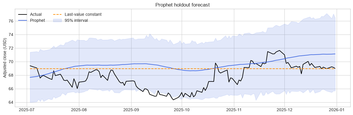

The black line is the observed adjusted close, the blue line is Prophet’s point forecast, and the shaded area is its nominal 95% interval. The orange dashed line shows the constant baseline that achieved lower errors on this holdout.

After evaluation, we fit a new model on all available observations and forecast 126 future weekdays. Prophet’s make_future_dataframe generates the requested calendar; freq="B" means Monday through Friday, not an exchange-specific calendar. It can therefore include market holidays such as New Year’s Day.

FORECAST_PERIODS = 126

final_model = fit_prophet(prophet_data)
future_dates = final_model.make_future_dataframe(periods=FORECAST_PERIODS, freq="B")
np.random.seed(RANDOM_SEED)
forecast_df = final_model.predict(future_dates)
future_forecast = forecast_df.loc[
  forecast_df["ds"] > prophet_data["ds"].max(),
  ["ds", "yhat_lower", "yhat", "yhat_upper"],
].copy()

figure = final_model.plot(forecast_df, figsize=(12, 5), include_legend=True)
axis = figure.axes[0]
axis.axvline(prophet_data["ds"].max(), color="black", linestyle="--", linewidth=1)
axis.set(title=f"{STOCK_NAME} forecast for {FORECAST_PERIODS} future weekdays", ylabel="Adjusted close (USD)")
figure.tight_layout()
plt.show()

future_forecast.tail()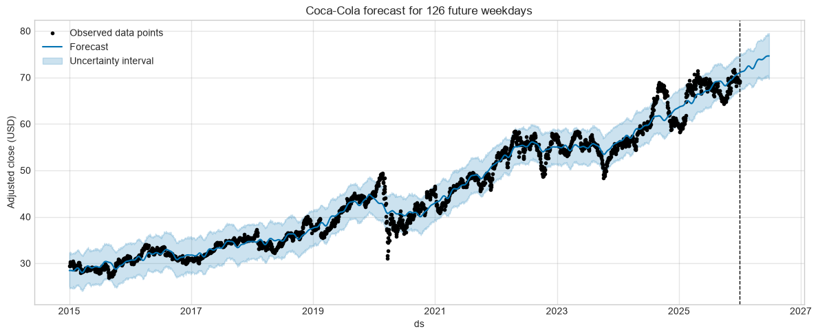

Step #5 Analyzing Model Components

We can gain a better understanding of the fitted components with plot_components. The figure shows the trend and the weekly and yearly seasonalities enabled by the available history.

components_figure = final_model.plot_components(
  forecast_df,
  weekly_start=0,
  figsize=(12, 8),
)
components_figure.suptitle("Prophet forecast components", y=1.02)
components_figure.tight_layout()
plt.show()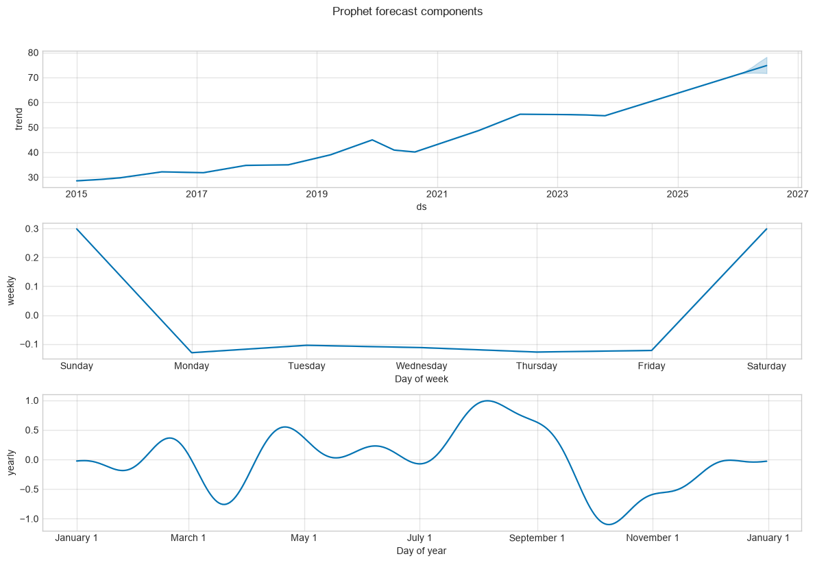

The trend is piecewise linear and can change slope at the fitted changepoints. Interpret the seasonal curves carefully: the historical stock data has no weekend observations, so Saturday and Sunday values in the weekly component are unsupported extrapolations. Seasonal patterns in historical prices also do not guarantee a repeatable trading opportunity.

Step #6 Adjusting the Changepoints of our Facebook Prophet Model

Let’s take a closer look at the changepoints in our model. Prophet places potential changepoints at evenly spaced quantiles of the selected history and regularizes their slope adjustments. The fitted model may use some adjustments strongly and shrink others toward zero. These points describe trend flexibility; they are not an outlier detector and do not guarantee a more accurate forecast.

6.1 Checking Current Changepoints

We can illustrate the changepoints in our model with the add_changepoints_to_plot method. The method adds vertical lines to a plot to indicate the locations of the changepoints in the data. By plotting the changepoints on a graph, we can visually identify when these changes in trend occur and potentially diagnose any issues with our model.

default_figure = final_model.plot(
  forecast_df,
  uncertainty=False,
  figsize=(12, 5),
  include_legend=True,
)
default_axis = default_figure.axes[0]
add_changepoints_to_plot(default_axis, final_model, forecast_df)
default_axis.set(
  title="Potential changepoints in the first 80% of the history",
  xlim=(prophet_data["ds"].max() - pd.DateOffset(years=5), future_dates["ds"].max()),
)
default_figure.tight_layout()
plt.show()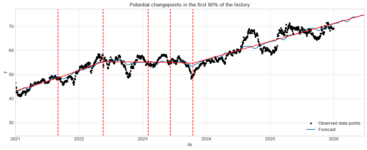

With the default changepoint_range=0.8, Prophet places its 25 potential changepoints across the first 80% of the training history. This leaves the final 20% available to reveal whether the latest fitted slope continues without adding more trend breaks.

6.2 Adjusting Changepoints

Setting changepoint_range=1.0 redistributes the same default number of potential changepoints across the complete history. It does not automatically add changepoints or give recent observations extra weight. Because this choice changes the extrapolated trend, it should be selected through validation rather than by choosing the most appealing future curve.

full_range_model = fit_prophet(prophet_data, changepoint_range=1.0)
np.random.seed(RANDOM_SEED)
full_range_forecast = full_range_model.predict(future_dates)

full_range_figure = full_range_model.plot(
  full_range_forecast,
  uncertainty=False,
  figsize=(12, 5),
  include_legend=True,
)
full_range_axis = full_range_figure.axes[0]
add_changepoints_to_plot(full_range_axis, full_range_model, full_range_forecast)
full_range_axis.set(
  title="Potential changepoints across the full history",
  xlim=(prophet_data["ds"].max() - pd.DateOffset(years=5), future_dates["ds"].max()),
)
full_range_figure.tight_layout()
plt.show()

pd.DataFrame(
  {
    "candidate_count": [len(final_model.changepoints), len(full_range_model.changepoints)],
    "latest_candidate": [final_model.changepoints.max(), full_range_model.changepoints.max()],
    "last_yhat": [forecast_df["yhat"].iloc[-1], full_range_forecast["yhat"].iloc[-1]],
  },
  index=["range=0.8", "range=1.0"],
)

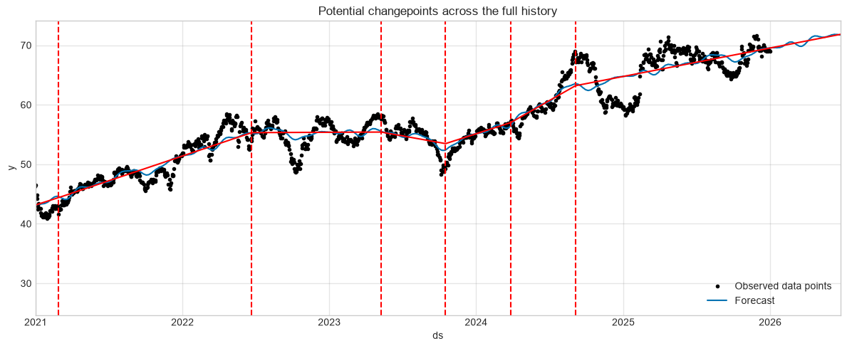
Both models still have 25 candidate dates, but the latest candidate moves from October 2023 to December 2025 and the final point forecasts differ. Manual changepoints can be supplied when constructing the model, for example Prophet(changepoints=["2020-03-23"]). Such dates should reflect defensible domain knowledge and still be validated out of sample.

Summary

In this article, we used Prophet to model Coca-Cola’s adjusted closing price. We prepared the required ds and y columns, created a chronological holdout, evaluated a nominal 95% uncertainty interval, and compared the model with a constant last-value baseline. We then refitted Prophet on all observations, generated a future weekday forecast, inspected its components, and compared two changepoint candidate windows.

Also: Mastering Multivariate Stock Market Prediction with Python

The holdout result is the most important lesson: Prophet did not beat the simple baseline on this period. Prophet remains useful because it is quick to fit, interpretable, and configurable, but complexity is not evidence of predictive value. Validate every forecasting choice on unseen dates and retain the simplest model that performs reliably.

Sources and Further Reading

1. Taylor and Letham, 2017, Forecasting at scale
2. Prophet documentation: Quick Start
3. David Forsyth (2019) Applied Machine Learning Springer

The links above to Amazon are affiliate links. By buying through these links, you support the Relataly.com blog and help to cover the hosting costs. Using the links does not affect the price.

Other Methods for Time Series Forecasting

• Univariate time series forecasting with Recurrent Neural Networks
• Multivariate time series forecasting with Recurrent Neural Networks
• Forecasting sales data with ARIMA models