Stock Market Forecasting Neural Networks for Multi-Output Regression in Python

Multi-output time series regression can forecast several steps of a time series at once. The number of neurons in the final output layer determines how many steps the model can predict. Models with one output return single-step forecasts. Models with various outputs can return entire series of time steps and thus deliver a more detailed projection of how a time series could develop in the future. This article is a hands-on Python tutorial that shows how to design a neural network architecture with multiple outputs. The goal is to create a multi-output model for stock-price forecasting using Python and Keras. By the end of this tutorial, you will have learned how to design a multi-output model for stock price forecasting using Python and Keras. This knowledge can be applied to other types of time series forecasting tasks, such as weather forecasting or sales forecasting.

This article proceeds as follows: We briefly discuss the architecture of a multi-output neural network. After familiarizing ourselves with the model architecture, we develop a Keras neural network for multi-output regression. For data preparation, we perform various steps, including cleaning, splitting, selecting, and scaling the data. Afterward, we define a model architecture with multiple LSTM layers and ten output neurons in the last layer. This architecture enables the model to generate projections for ten consecutive steps. After configuring the model architecture, we train the model with the historical daily prices of the Apple stock. Finally, we use this model to generate a ten-day forecast.

Disclaimer

This article does not constitute financial advice. Stock markets can be very volatile and are generally difficult to predict. Predictive models and other forms of analytics applied in this article only serve the purpose of illustrating machine learning use cases.

Multi-Output Regression vs. Single-Output Regression

In time series regression, we train a statistical model on the past values of a time series to make statements about how the time series develops further. During model training, we feed the model with so-called mini-batches and the corresponding target values. The model then creates forecasts for all input batches and compares these predictions to the actual target values to calculate the residuals (prediction errors). In this way, the model can adjust its parameters iteratively and learn to make better predictions.

Multivariate forecasting models take into account multiple input variables, such as historical time series data and additional features like moving averages or momentum indicators, to improve the accuracy of their predictions. The idea is that these various variables can help the model identify patterns in the data that suggest future price movements.

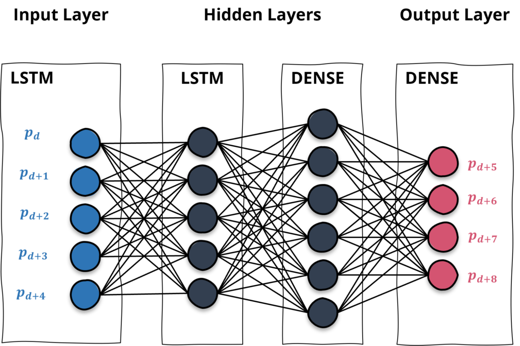
An exemplary architecture of a neural network with five input neurons (blue) and four output neurons (red)

The Architecture of a Neural Network with Multiple Outputs

Next, we will discuss the architecture of a neural network with multiple outputs. The architecture consists of several layers, including an input layer, several hidden layers, and an output layer. The number of neurons in the first layer must match the input data, and the number of neurons in the output layer determines the period length of the predictions.

Models with a single neuron in the output layer are used to predict a single time step. It is possible to predict multiple price steps with a single-output model. It requires a rolling forecasting approach in which the outputs are iteratively reused to make further-reaching predictions. However, this way is somewhat cumbersome. A more elegant way is to train a multi-output model right away.

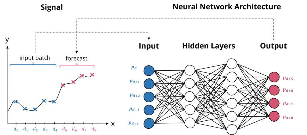
The inputs and outputs of a neural network for time series regression with five input neurons and four outputs

Training Neural Networks with Multiple Outputs

A model with multiple neurons in the output layer can predict numerous steps once per batch. Multi-output regression models train on many sequences of subsequent values, followed by the consecutive output sequence. The model architecture thus contains multiple neurons in the initial layer and various neurons in the output layer (as illustrated).

In a multi-output regression model, each neuron in the output layer is responsible for predicting a different time step in the future. To train such a model, you need to provide a sequence of input data followed by the corresponding sequence of output data. For example, if you want to predict the stock price for the next ten days, you would provide a sequence of input data containing the historical stock prices for the past 50 days, followed by a sequence of output data containing the stock prices for the next 10 days.

The model will then learn to map the input sequence to the output sequence so that it can make predictions for multiple time steps in the future based on the input data.

In the next part of this tutorial, we will walk through the process of developing a multi-output regression model in more detail.

Implementing a Neural Network Model for Multi-Output Multi-Step Regression in Python

Let’s get started with the hands-on Python part. In the following, we will develop a neural network with Keras and Tensorflow that forecasts the Apple stock price. To prepare the data for a neural network with multiple outputs in time series forecasting, we will spend the most time preparing it and bringing it into the right shape. Broadly this involves the following steps:

1. Load the time series data that we want to use as input and output for your model. We use historical price data that is available via the yahoo finance API.
2. Then we split our data into training and testing sets. We will use the training set to fit the model and the testing set to evaluate the model’s performance.
3. Preprocess the data: This includes scaling the data and selecting relevant features.
4. Reshape the data and bring them into a format that can be input into the neural network. This involves converting the data into a 3D array for time series data.
5. Finally, we will train our model and generate the forecasting.

The code is available on the GitHub repository.

Neural network architectures with multiple outputs allow for more potent solutions but are more complex to train. Image created with Midjourney.

Prerequisites

Before beginning the coding part, ensure that you have set up your Python 3 environment and required packages. If you don’t have a Python environment, consider Anaconda. To set it up, you can follow the steps in this tutorial.

Also, make sure you install all required packages. In this tutorial, we will be working with the following standard packages:

• pandas
• NumPy
• matplotlib

In addition, we will be using the machine learning libraries Keras, Scikit-learn, and Tensorflow. For visualization, we will be using the Seaborn package.

Please also have either the pandas_datareader or the yfinance package installed. You will use one of these packages to retrieve the historical stock quotes.

You can install these packages using console commands:

• pip install
• conda install  (if you are using the anaconda packet manager)

Step #1: Load the Data

The Pandas DataReader library is our first choice for interacting with the yahoo finance API. If the library causes a problem (it sometimes does), you can also use the yfinance package, which should return the same data. We begin by loading historical price quotes of the Apple stock from the public yahoo finance API. Running the code below will load the data into a Pandas DataFrame.

# import pandas_datareader as webreader # Remote data access for pandas
import math # Mathematical functions
import numpy as np # Fundamental package for scientific computing with Python
import pandas as pd # Additional functions for analysing and manipulating data
from datetime import date, timedelta, datetime # Date Functions
from pandas.plotting import register_matplotlib_converters # This function adds plotting functions for calender dates
import matplotlib.pyplot as plt # Important package for visualization - we use this to plot the market data
import matplotlib.dates as mdates # Formatting dates
from sklearn.metrics import mean_absolute_error, mean_squared_error # Packages for measuring model performance / errors
from keras.models import Sequential # Deep learning library, used for neural networks
from keras.layers import LSTM, Dense, Dropout # Deep learning classes for recurrent and regular densely-connected layers
from keras.callbacks import EarlyStopping # EarlyStopping during model training
from sklearn.preprocessing import RobustScaler, MinMaxScaler # This Scaler removes the median and scales the data according to the quantile range to normalize the price data
import seaborn as sns

# from pandas_datareader.nasdaq_trader import get_nasdaq_symbols
# symbols = get_nasdaq_symbols()

# Setting the timeframe for the data extraction
today = date.today()
date_today = today.strftime("%Y-%m-%d")
date_start = '2010-01-01'

# Getting NASDAQ quotes
stockname = 'Apple'
symbol = 'AAPL'
# df = webreader.DataReader(
#     symbol, start=date_start, end=date_today, data_source="yahoo"
# )

import yfinance as yf #Alternative package if webreader does not work: pip install yfinance
df = yf.download(symbol, start=date_start, end=date_today)

# # Create a quick overview of the dataset
df.head()

Tensorflow Version: 2.6.0
Num GPUs: 1
[*********************100%***********************]  1 of 1 completed
			Open		High		Low			Close		Adj Close	Volume
Date
2010-01-04	7.622500	7.660714	7.585000	7.643214	6.515213	493729600
2010-01-05	7.664286	7.699643	7.616071	7.656429	6.526477	601904800
2010-01-06	7.656429	7.686786	7.526786	7.534643	6.422666	552160000
2010-01-07	7.562500	7.571429	7.466071	7.520714	6.410791	477131200
2010-01-08	7.510714	7.571429	7.466429	7.570714	6.453413	447610800

The data should comprise the following columns:

• Close
• Open
• High
• Low
• Adj Close
• Volume

The target variable that we are trying to predict is the Closing price (Close).

Step #2: Explore the Data

Once we have loaded the data, we print a quick overview of the time-series data using different line graphs. The following code will plot a line chart for each column in df_plot using the seaborn library. The charts will be organized in a grid with nrows number of rows and ncols number of columns. The sharex parameter is set to True, which means that the x-axes of the subplots will be shared. The figsize parameter determines the size of the plot in inches.

# Plot line charts
df_plot = df.copy()

ncols = 2
nrows = int(round(df_plot.shape[1] / ncols, 0))

fig, ax = plt.subplots(nrows=nrows, ncols=ncols, sharex=True, figsize=(14, 7))
for i, ax in enumerate(fig.axes):
        sns.lineplot(data = df_plot.iloc[:, i], ax=ax)
        ax.tick_params(axis="x", rotation=30, labelsize=10, length=0)
        ax.xaxis.set_major_locator(mdates.AutoDateLocator())
fig.tight_layout()
plt.show()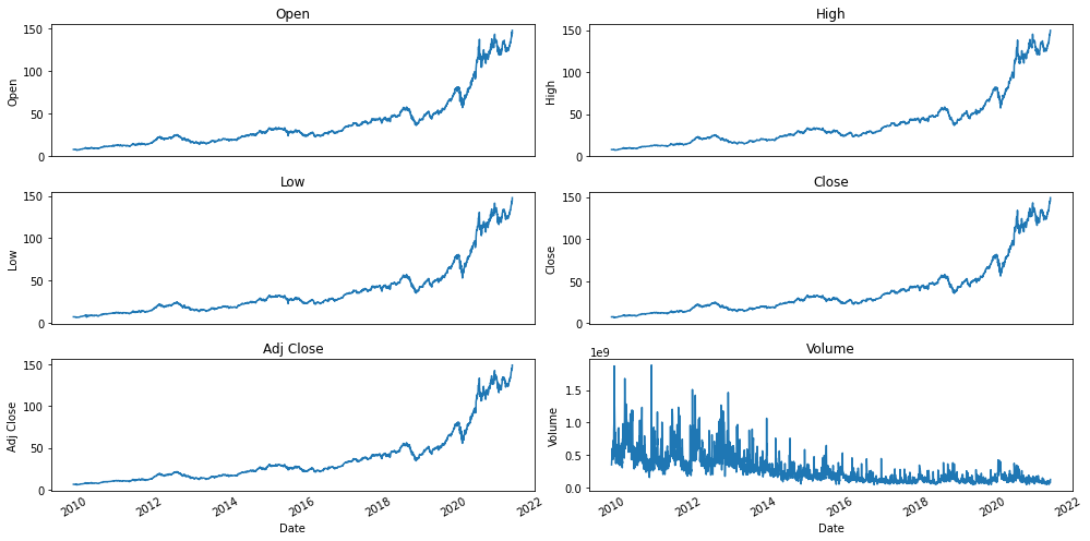

The line plots look as expected and reflect the Apple stock price history. Because we are fetching daily data from an API, please note that the lineplots will look different depending on when you run the code.

Step #3: Preprocess the Data

Next, we prepare the data for the training process of our multi-output forecasting model. Preparing the data for multivariate forecasting involves several steps:

• Selecting features for model training
• Scaling and splitting the data into separate sets for training and testing
• Slicing the time series into several shifted training batches

Remember that the steps are specific to our data and the use case. The steps required to prepare the data for a neural network with multiple outputs in time series forecasting will depend on the characteristics of your data and the requirements of your model. It is essential to consider these factors and tailor your data preparation accordingly and carefully.

3.1 Basic Preparations

We begin by creating a copy of the initial data and resetting the index.

# Indexing Batches
df_train = df.sort_values(by=['Date']).copy()

# We safe a copy of the dates index, before we need to reset it to numbers
date_index = df_train.index

# We reset the index, so we can convert the date-index to a number-index
df_train = df_train.reset_index(drop=True).copy()
df_train.head(5)

			Open		High		Low			Close		Adj Close	Volume
Date
2022-11-29	144.289993	144.809998	140.350006	141.169998	141.169998	83763800
2022-11-30	141.399994	148.720001	140.550003	148.029999	148.029999	111224400
2022-12-01	148.210007	149.130005	146.610001	148.309998	148.309998	71250400
2022-12-02	145.960007	148.000000	145.649994	147.809998	147.809998	65421400
2022-12-05	147.770004	150.919998	145.770004	146.630005	146.630005	68732400

3.2 Feature Selection and Scaling

We proceed with feature selection. To keep things simple, we will use the features from the input data without any modifications. After selecting the features, we scale them to a range between 0 and 1. To ease unscaling the predictions after training, we create two different scalers: One for the training data, which takes five columns, and one for the output data that scales a single column (the Close Price). I have covered feature engineering in a separate article if you want to learn more about this topic.

def prepare_data(df):

    # List of considered Features
    FEATURES = ['Open', 'High', 'Low', 'Close', 'Volume']

    print('FEATURE LIST')
    print([f for f in FEATURES])

    # Create the dataset with features and filter the data to the list of FEATURES
    df_filter = df[FEATURES]

    # Convert the data to numpy values
    np_filter_unscaled = np.array(df_filter)
    #np_filter_unscaled = np.reshape(np_unscaled, (df_filter.shape[0], -1))
    print(np_filter_unscaled.shape)

    np_c_unscaled = np.array(df['Close']).reshape(-1, 1)

    return np_filter_unscaled, np_c_unscaled, df_filter

np_filter_unscaled, np_c_unscaled, df_filter = prepare_data(df_train)

# Creating a separate scaler that works on a single column for scaling predictions
# Scale each feature to a range between 0 and 1
scaler_train = MinMaxScaler()
np_scaled = scaler_train.fit_transform(np_filter_unscaled)

# Create a separate scaler for a single column
scaler_pred = MinMaxScaler()
np_scaled_c = scaler_pred.fit_transform(np_c_unscaled)

FEATURE LIST
['Open', 'High', 'Low', 'Close', 'Volume']
(3254, 5)

The final step of the data preparation is to create the structure for the input data. This structure needs to match the input layer of the model architecture.

3.3 Slicing the Data for a Model with Multiple In- and Outputs

The code below starts a sliding window process that cuts the initial time series data into multiple slices, i.e., mini-batches. Each batch is a smaller fraction of the initial time series shifted by a single step. Because we will feed our model with multivariate input data, the time series consists of five input columns/features. Each batch comprises a period of 50 steps from the time series and an output sequence of ten consecutive values. To validate that the batches have the right shape, we visualize mini-batches in a line graph with their consecutive target values.

# Set the input_sequence_length length - this is the timeframe used to make a single prediction
input_sequence_length = 50
# The output sequence length is the number of steps that the neural network predicts
output_sequence_length = 10 #

# Prediction Index
index_Close = df_train.columns.get_loc("Close")

# Split the training data into train and train data sets
# As a first step, we get the number of rows to train the model on 80% of the data
train_data_length = math.ceil(np_scaled.shape[0] * 0.8)

# Create the training and test data
train_data = np_scaled[:train_data_length, :]
test_data = np_scaled[train_data_length - input_sequence_length:, :]

# The RNN needs data with the format of [samples, time steps, features]
# Here, we create N samples, input_sequence_length time steps per sample, and f features
def partition_dataset(input_sequence_length, output_sequence_length, data):
    x, y = [], []
    data_len = data.shape[0]
    for i in range(input_sequence_length, data_len - output_sequence_length):
        x.append(data[i-input_sequence_length:i,:]) #contains input_sequence_length values 0-input_sequence_length * columns
        y.append(data[i:i + output_sequence_length, index_Close]) #contains the prediction values for validation (3rd column = Close),  for single-step prediction

    # Convert the x and y to numpy arrays
    x = np.array(x)
    y = np.array(y)
    return x, y

# Generate training data and test data
x_train, y_train = partition_dataset(input_sequence_length, output_sequence_length, train_data)
x_test, y_test = partition_dataset(input_sequence_length, output_sequence_length, test_data)

# Print the shapes: the result is: (rows, training_sequence, features) (prediction value, )
print(x_train.shape, y_train.shape)
print(x_test.shape, y_test.shape)

# Validate that the prediction value and the input match up
# The last close price of the second input sample should equal the first prediction value
nrows = 3 # number of shifted plots
fig, ax = plt.subplots(nrows=nrows, ncols=1, figsize=(16, 8))
for i, ax in enumerate(fig.axes):
    xtrain = pd.DataFrame(x_train[i][:,index_Close], columns={f'x_train_{i}'})
    ytrain = pd.DataFrame(y_train[i][:output_sequence_length-1], columns={f'y_train_{i}'})
    ytrain.index = np.arange(input_sequence_length, input_sequence_length + output_sequence_length-1)
    xtrain_ = pd.concat([xtrain, ytrain[:1].rename(columns={ytrain.columns[0]:xtrain.columns[0]})])
    df_merge = pd.concat([xtrain_, ytrain])
    sns.lineplot(data = df_merge, ax=ax)
plt.show

(2544, 50, 5) (2544, 10)
(640, 50, 5) (640, 10)
<function matplotlib.pyplot.show(close=None, block=None)>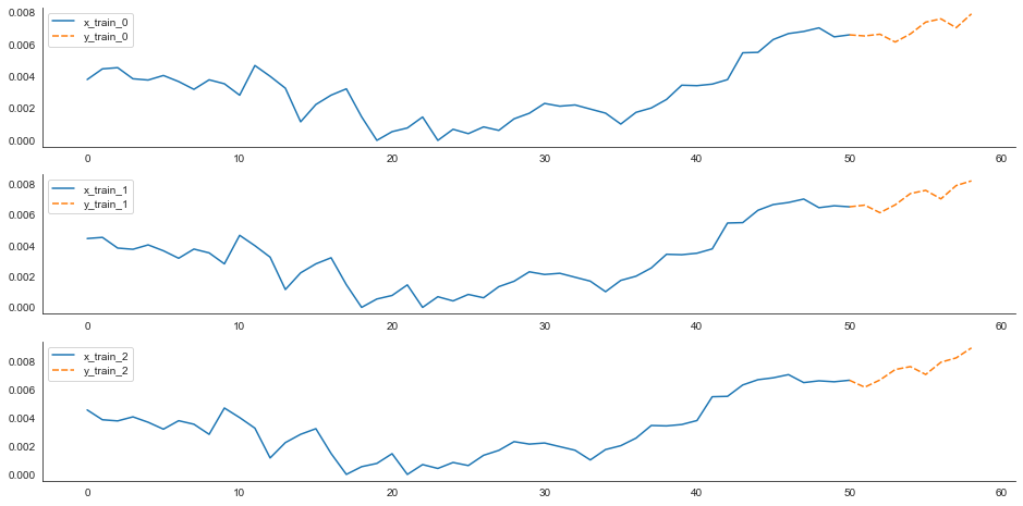

Step #4: Prepare the Neural Network Architecture and Train the Multi-Output Regression Model

Now that we have the training data prepared and ready, the next step is to configure the architecture of the multi-out neural network. Because we will be using multiple input series, our model is, in fact, a multivariate architecture so that it corresponds to the input training batches.

4.1 Configuring and Training the Model

We choose a comparably simple architecture with only two LSTM layers and two additional dense layers. The first dense layer has 20 neurons, and the second layer is the output layer, which has ten output neurons. If you wonder how I got to the number of neurons in the third layer, I conducted several experiments and found that this number leads to solid results.

To ensure that the architecture matches our input data’s structure, we reuse the variables for the previous code section (n_input_neurons, n_output_neurons. The input sequence length is 50, and the output sequence (the steps for the period we want to predict) is ten.

# Configure the neural network model
model = Sequential()
n_output_neurons = output_sequence_length

# Model with n_neurons = inputshape Timestamps, each with x_train.shape[2] variables
n_input_neurons = x_train.shape[1] * x_train.shape[2]
print(n_input_neurons, x_train.shape[1], x_train.shape[2])
model.add(LSTM(n_input_neurons, return_sequences=True, input_shape=(x_train.shape[1], x_train.shape[2])))
model.add(LSTM(n_input_neurons, return_sequences=False))
model.add(Dense(20))
model.add(Dense(n_output_neurons))

# Compile the model
model.compile(optimizer='adam', loss='mse')

After configuring the model architecture, we can initiate the training process and illustrate how the loss develops over the training epochs.

# Training the model
epochs = 10
batch_size = 16
early_stop = EarlyStopping(monitor='loss', patience=5, verbose=1)
history = model.fit(x_train, y_train,
                    batch_size=batch_size,
                    epochs=epochs,
                    validation_data=(x_test, y_test)
                   )

                    #callbacks=[early_stop])

Epoch 1/5
159/159 [==============================] - 7s 14ms/step - loss: 0.0047 - val_loss: 0.0262
Epoch 2/5
159/159 [==============================] - 2s 11ms/step - loss: 3.6759e-04 - val_loss: 0.0097
Epoch 3/5
159/159 [==============================] - 2s 11ms/step - loss: 1.5222e-04 - val_loss: 0.0056
Epoch 4/5
159/159 [==============================] - 2s 11ms/step - loss: 1.0327e-04 - val_loss: 0.0031
Epoch 5/5
159/159 [==============================] - 2s 11ms/step - loss: 1.1690e-04 - val_loss: 0.0026

4.2 Loss Curve

Next, we plot the loss curve, which represents the amount of error between the model’s predicted values and the actual values in the training data. A lower loss value indicates that the model makes more accurate predictions on the training data.

# Plot training & validation loss values
fig, ax = plt.subplots(figsize=(10, 5), sharex=True)
plt.plot(history.history["loss"])
plt.title("Model loss")
plt.ylabel("Loss")
plt.xlabel("Epoch")
ax.xaxis.set_major_locator(plt.MaxNLocator(epochs))
plt.legend(["Train", "Test"], loc="upper left")
plt.grid()
plt.show()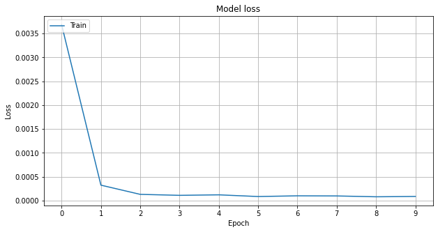

As we can see, the loss curve drops quickly during training, which typically means that the model is quickly learning to make accurate predictions.

Step #5 Evaluate Model Performance

Now that we have trained the model, we can make forecasts on the test data and use traditional regression metrics such as the MAE, MAPE, or MDAPE to measure the performance of our model.

# Get the predicted values
y_pred_scaled = model.predict(x_test)

# Unscale the predicted values
y_pred = scaler_pred.inverse_transform(y_pred_scaled)
y_test_unscaled = scaler_pred.inverse_transform(y_test).reshape(-1, output_sequence_length)

# Mean Absolute Error (MAE)
MAE = mean_absolute_error(y_test_unscaled, y_pred)
print(f'Median Absolute Error (MAE): {np.round(MAE, 2)}')

# Mean Absolute Percentage Error (MAPE)
MAPE = np.mean((np.abs(np.subtract(y_test_unscaled, y_pred)/ y_test_unscaled))) * 100
print(f'Mean Absolute Percentage Error (MAPE): {np.round(MAPE, 2)} %')

# Median Absolute Percentage Error (MDAPE)
MDAPE = np.median((np.abs(np.subtract(y_test_unscaled, y_pred)/ y_test_unscaled)) ) * 100
print(f'Median Absolute Percentage Error (MDAPE): {np.round(MDAPE, 2)} %')

def prepare_df(i, x, y, y_pred_unscaled):
    # Undo the scaling on x, reshape the testset into a one-dimensional array, so that it fits to the pred scaler
    x_test_unscaled_df = pd.DataFrame(scaler_pred.inverse_transform((x[i]))[:,index_Close]).rename(columns={0:'x_test'})

    y_test_unscaled_df = []
    # Undo the scaling on y
    if type(y) == np.ndarray:
        y_test_unscaled_df = pd.DataFrame(scaler_pred.inverse_transform(y)[i]).rename(columns={0:'y_test'})

    # Create a dataframe for the y_pred at position i, y_pred is already unscaled
    y_pred_df = pd.DataFrame(y_pred_unscaled[i]).rename(columns={0:'y_pred'})
    return x_test_unscaled_df, y_pred_df, y_test_unscaled_df

def plot_multi_test_forecast(x_test_unscaled_df, y_test_unscaled_df, y_pred_df, title):
    # Package y_pred_unscaled and y_test_unscaled into a dataframe with columns pred and true
    if type(y_test_unscaled_df) == pd.core.frame.DataFrame:
        df_merge = y_pred_df.join(y_test_unscaled_df, how='left')
    else:
        df_merge = y_pred_df.copy()

    # Merge the dataframes
    df_merge_ = pd.concat([x_test_unscaled_df, df_merge]).reset_index(drop=True)

    # Plot the linecharts
    fig, ax = plt.subplots(figsize=(20, 8))
    plt.title(title, fontsize=12)
    ax.set(ylabel = stockname + "_stock_price_quotes")
    sns.lineplot(data = df_merge_, linewidth=2.0, ax=ax)

# Creates a linechart for a specific test batch_number and corresponding test predictions
batch_number = 50
x_test_unscaled_df, y_pred_df, y_test_unscaled_df = prepare_df(i, x_test, y_test, y_pred)
title = f"Predictions vs y_test - test batch number {batch_number}"
plot_multi_test_forecast(x_test_unscaled_df, y_test_unscaled_df, y_pred_df, title)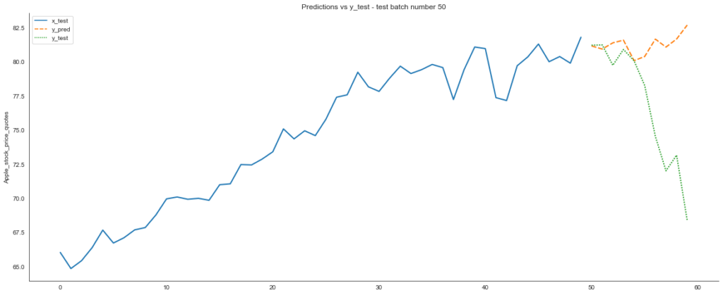

The quality of the predictions is acceptable, considering that this tutorial aimed not to achieve excellent predictions but to demonstrate the process and architecture of training a multi-output regression. So, there is certainly room for improvement. Feel free to experiment with different features or try other hyperparameters and neural network layers.

Step #6 Create a New Forecast

Finally, let’s create a forecast on a new dataset. We take the scaled dataset from section 2 (np_scaled) and extract a series with the latest 50 values. The data is reshaped into a 3D array with shape (1, 50, 5) to match the expected input shape of the model. We use these values to generate a new prediction for the next ten days using the predict method. We store the result in the y_pred_scaled variable. In addition, we need to transform the predictions back to the original scale. We do this by using the inverse_transform method of the scaler_pred object, which was fit on the training data. Finally, we visualize the multi-step forecast in another line chart.

# Get the latest input batch from the test dataset, which is contains the price values for the last ten trading days
x_test_latest_batch = np_scaled[-50:,:].reshape(1,50,5)

# Predict on the batch
y_pred_scaled = model.predict(x_test_latest_batch)
y_pred_unscaled = scaler_pred.inverse_transform(y_pred_scaled)

# Prepare the data and plot the input data and the predictions
x_test_unscaled_df, y_test_unscaled_df, _ = prepare_df(0, x_test_latest_batch, '', y_pred_unscaled)
plot_multi_test_forecast(x_test_unscaled_df, '', y_test_unscaled_df, "x_new Vs. y_new_pred")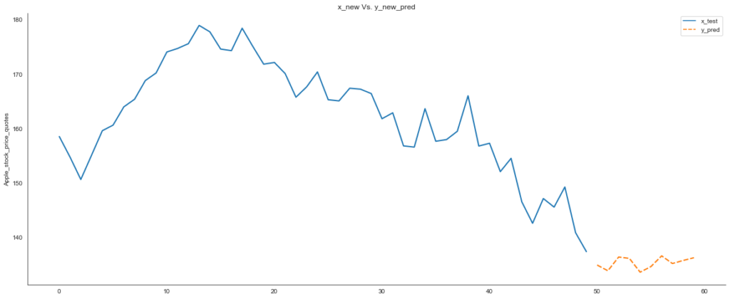

Summary

In this tutorial, we demonstrated how to use multiple output neural networks to make predictions at different time steps. We first discussed the architecture of a recurrent neural network and how it can be used to process sequential data. We then showed how to properly preprocess the data and split it into training and test sets for training a multi-output regression model.

Next, we trained a model to predict the stock price of Apple ten steps into the future using historical data. We also discussed how to use the trained model to make multi-step predictions on new data and how to visualize the results.

To further improve the performance of the model, you can experiment with different hyperparameters and adjust the model architecture. For example, adding more neurons to the output layers will increase the prediction horizon, but remember that prediction error will also increase as the horizon lengthens. You can also try using different activation functions or adding more layers to the model to see how it affects the performance.

I hope this article was helpful in understanding multi-output neural networks better. If you have any questions or comments, please let me know.

Sources and Further Reading

1. Charu C. Aggarwal (2018) Neural Networks and Deep Learning
2. Jansen (2020) Machine Learning for Algorithmic Trading: Predictive models to extract signals from market and alternative data for systematic trading strategies with Python
3. Aurélien Géron (2019) Hands-On Machine Learning with Scikit-Learn, Keras, and TensorFlow: Concepts, Tools, and Techniques to Build Intelligent Systems
4. David Forsyth (2019) Applied Machine Learning Springer
5. Andriy Burkov (2020) Machine Learning Engineering

The links above to Amazon are affiliate links. By buying through these links, you support the Relataly.com blog and help to cover the hosting costs. Using the links does not affect the price.

If you want to learn about an alternative approach to univariate stock market forecasting, consider taking a look at Facebook Prophet or ARIMA models